Tasche: Euler risk allocation

A bank’s capital is set for the whole portfolio, but desks must be charged for their share. Because VaR, ES and volatility are positively homogeneous in the position sizes, Euler’s theorem splits them exactly:

\[\rho(w) = \sum_i w_i \frac{\partial \rho}{\partial w_i}.\]

Tasche (1999) proved that these Euler contributions are the only allocation under which growing a position with an above-average return on risk capital improves the whole portfolio’s. A hedge gets a negative contribution: it releases capital.

import matplotlib.pyplot as plt
import numpy as np

from financialkit.risk import euler_allocation, expected_shortfall, scenario_es_allocation
from financialkit.risk.visualizers import plot_allocation

labels = ["equities", "credit", "rates", "FX hedge"]
w = np.array([40.0, 30.0, 50.0, 15.0])  # $m
vols = np.array([0.012, 0.008, 0.004, 0.006])
corr = np.array([[1.0, 0.6, -0.2, 0.3], [0.6, 1.0, 0.0, 0.2], [-0.2, 0.0, 1.0, -0.1], [0.3, 0.2, -0.1, 1.0]])
cov = corr * np.outer(vols, vols)
w[3] = -w[3]  # the hedge is short

Normal VaR and ES contributions

fig, axes = plt.subplots(1, 2, figsize=(11, 4))
for ax, m in zip(axes, ("var", "es"), strict=True):
    res = euler_allocation(w, cov, 0.99, m)
    plot_allocation(res, labels, ax=ax)
    print(f"{m}: " + ", ".join(f"{lbl} {c:.3f}" for lbl, c in zip(labels, res.contributions, strict=True)) + f"; total {res.total:.3f}")
fig.tight_layout()

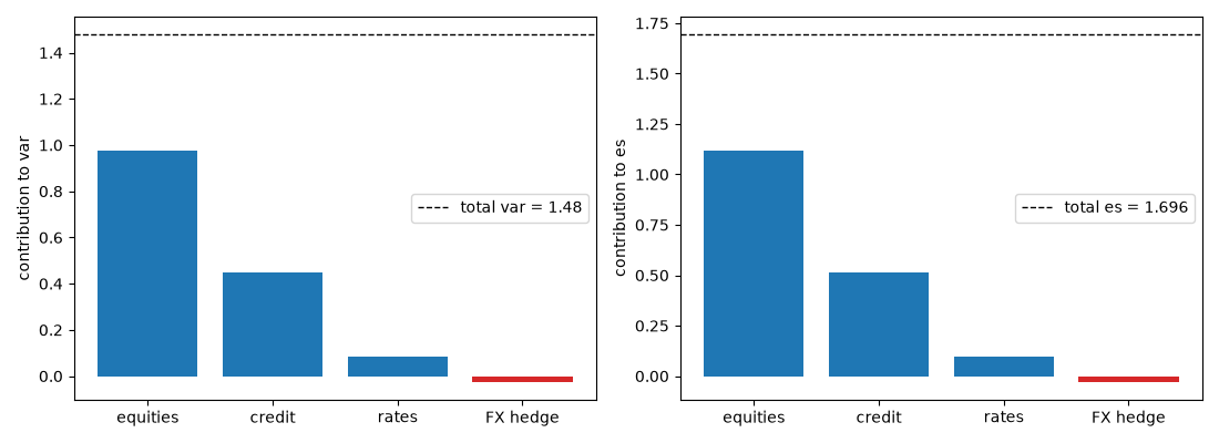
var: equities 0.977, credit 0.447, rates 0.083, FX hedge -0.027; total 1.480
es: equities 1.120, credit 0.513, rates 0.095, FX hedge -0.031; total 1.696

Scenario-based ES contributions

With fat-tailed scenarios, each position’s contribution is minus its average P&L in the portfolio’s worst 1% of days, and they still add up to the portfolio’s ES.

rng = np.random.default_rng(0)
nu = 4
Z = rng.multivariate_normal(np.zeros(4), corr, 20_000) / np.sqrt(rng.chisquare(nu, (20_000, 1)) / (nu - 2))
pnl = Z * vols * w
res = scenario_es_allocation(pnl, 0.99)
print(f"scenario ES {res.total:.3f} (portfolio ES {expected_shortfall(pnl.sum(axis=1), 0.99):.3f})")
print("shares: " + ", ".join(f"{lbl} {s:.0%}" for lbl, s in zip(labels, res.shares, strict=True)))

plt.show()

scenario ES 2.275 (portfolio ES 2.275)
shares: equities 68%, credit 29%, rates 5%, FX hedge -2%