Acerbi-Tasche expected shortfall

“The average loss beyond VaR” sounds like one number but is several when the distribution has atoms, as every sample does, and some versions are not coherent. Acerbi and Tasche (2002) gave the definition that is: average exactly the worst fraction \(p = 1 - \alpha\) of outcomes, charging only part of the atom at the quantile,

\[\mathrm{ES} = -\frac{1}{np}\Big(\sum_{i=1}^{\lfloor np \rfloor} X_{(i)} + (np - \lfloor np \rfloor) X_{(\lfloor np \rfloor + 1)}\Big).\]

In 2016 the Basel Committee’s Fundamental Review of the Trading Book replaced 99% VaR by 97.5% ES.

import matplotlib.pyplot as plt
import numpy as np

from financialkit.risk import expected_shortfall, historical_var, parametric_es, parametric_var

A discrete example

With 100 outcomes and a 2.5% tail, the estimator takes the two worst in full and half of the third. The naive “mean of losses at or beyond VaR” would average three.

x = -np.arange(1.0, 101.0)
print(f"VaR {historical_var(x, 0.975).var}, Acerbi-Tasche ES {expected_shortfall(x, 0.975)}, naive tail mean {-np.mean(np.sort(x)[:3]):.1f}")

VaR 98.0, Acerbi-Tasche ES 99.2, naive tail mean 99.0

Convergence to the closed form

For normal and Student-t profit and loss, the sample estimator converges to the closed forms, and the Basel 97.5% ES is close to the old 99% VaR for the normal but larger under fat tails.

rng = np.random.default_rng(0)
nu = 4
sizes = np.geomspace(250, 100_000, 12).astype(int)
fig, ax = plt.subplots(figsize=(7, 4))
for name, draw, exact in [
    ("normal", lambda k: rng.standard_normal(k), parametric_es(0.0, 1.0, 0.975)),
    ("Student-t(4)", lambda k: rng.standard_t(nu, k) / np.sqrt(nu / (nu - 2)), parametric_es(0.0, 1.0, 0.975, distribution="t", df=nu)),
]:
    est = np.array([[expected_shortfall(draw(k), 0.975) for _ in range(20)] for k in sizes])
    line = ax.errorbar(sizes, est.mean(axis=1), yerr=est.std(axis=1), fmt="o-", ms=3, capsize=2, label=f"{name} sample ES")
    ax.axhline(exact, color=line[0].get_color(), ls="--", lw=1)
ax.set_xscale("log")
ax.set_xlabel("sample size")
ax.set_ylabel("97.5% expected shortfall")
ax.legend()
fig.tight_layout()

for name, kw in [("normal", {}), ("t(4)", {"distribution": "t", "df": nu})]:
    print(f"{name:7s} 97.5% ES {parametric_es(0.0, 1.0, 0.975, **kw):.3f} vs 99% VaR {parametric_var(0.0, 1.0, 0.99, **kw):.3f}")

plt.show()

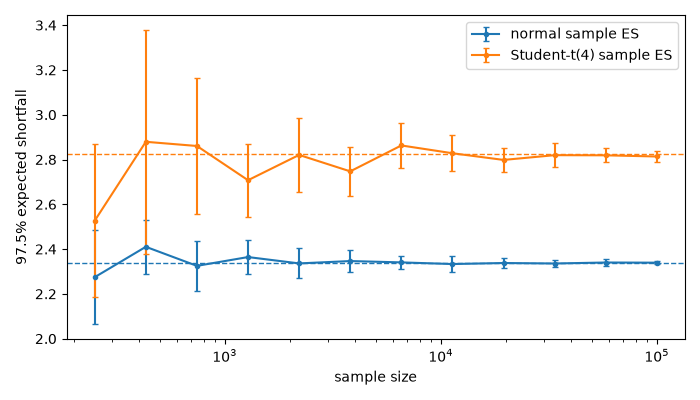
normal  97.5% ES 2.338 vs 99% VaR 2.326
t(4)    97.5% ES 2.824 vs 99% VaR 2.649