Carr and Madan’s FFT

Carr and Madan (1999) noticed that the call price, as a function of the log strike \(k\), is not integrable, but \(e^{\alpha k} C(k)\) is, and that its Fourier transform is a simple expression in the characteristic function. One fast Fourier transform then prices calls at thousands of strikes at once, for any model with a known characteristic function. The grids are linked: integration spacing \(\eta\) and strike spacing \(\lambda\) satisfy \(\lambda\eta = 2\pi/N\).

import matplotlib.pyplot as plt
import numpy as np

from financialkit.options import black_scholes_price
from financialkit.stochastic_volatility import BlackScholesModel, HestonModel, carr_madan_fft, carr_madan_price, lewis_price

S, T, r = 100.0, 1.0, 0.03

A whole strike grid from one FFT

bs = carr_madan_fft(BlackScholesModel(0.2), S, T, r)
mid = (bs.strikes > 50) & (bs.strikes < 200)
err = np.abs(bs.calls[mid] - black_scholes_price(S, bs.strikes[mid], T, r, 0.2))
print(f"{mid.sum()} strikes between 50 and 200, max error against Black-Scholes {err.max():.1e}")

heston = HestonModel(0.04, 1.5, 0.04, 0.5, -0.7)
res = carr_madan_fft(heston, S, T, r)
fig, (ax1, ax2) = plt.subplots(1, 2, figsize=(10, 4))
ax1.plot(res.strikes[mid], res.calls[mid], label="Heston, FFT")
ax1.plot(bs.strikes[mid], bs.calls[mid], "--", label="Black-Scholes 20%")
ax1.set_xlabel("strike K")
ax1.set_ylabel("call price")
ax1.legend()

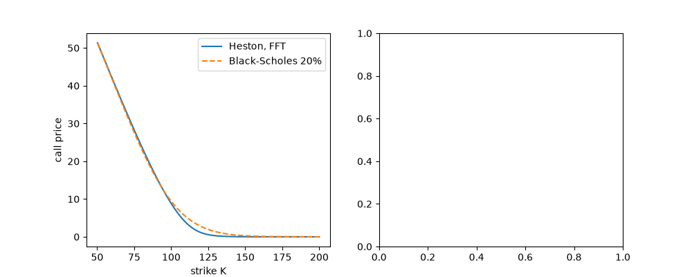
226 strikes between 50 and 200, max error against Black-Scholes 2.2e-07

<matplotlib.legend.Legend object at 0x116f57b60>

The damping exponent

Too little damping and the integrand is large near \(v = 0\); too much and the payoff’s growth is amplified. Mid-range values of \(\alpha\) are accurate to many digits.

K = np.array([80.0, 100.0, 120.0])
ref = np.asarray(lewis_price(heston, S, K, T, r))
alphas = np.linspace(0.1, 8.0, 40)
errors = [np.max(np.abs(carr_madan_price(heston, S, K, T, r, alpha=a) - ref)) for a in alphas]
ax2.semilogy(alphas, errors, marker="o", ms=3)
ax2.set_xlabel("damping alpha")
ax2.set_ylabel("max error at K = 80, 100, 120")
fig.tight_layout()

plt.show()