Fang and Oosterlee’s COS method

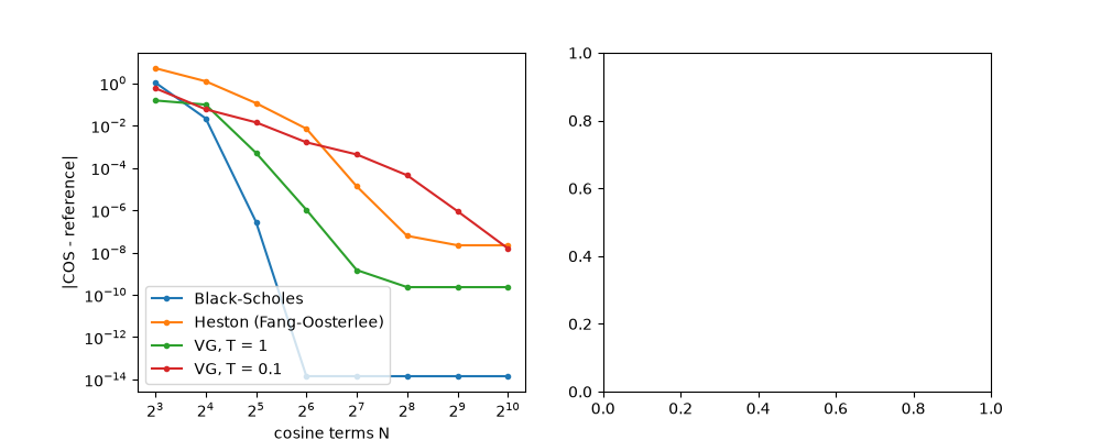
Fang and Oosterlee (2008) truncated the density of the log return to an interval \([a, b]\) set by its cumulants and expanded it in a cosine series, whose coefficients are read directly off the characteristic function. The payoff’s cosine coefficients are closed form, so a price is a dot product of two short vectors. For smooth densities the error falls exponentially with the number of terms; for a density with a kink, like short-dated variance gamma, only algebraically.

import matplotlib.pyplot as plt
import numpy as np

from financialkit.stochastic_volatility import BlackScholesModel, HestonModel, VarianceGammaModel, cos_density, cos_price, lewis_price

N = 2 ** np.arange(3, 11)
cases = {
    "Black-Scholes": (BlackScholesModel(0.25), 100.0, 1.0, 0.0),
    "Heston (Fang-Oosterlee)": (HestonModel(0.0175, 1.5768, 0.0398, 0.5751, -0.5711), 100.0, 1.0, 0.0),
    "VG, T = 1": (VarianceGammaModel(0.12, 0.2, -0.14), 90.0, 1.0, 0.1),
    "VG, T = 0.1": (VarianceGammaModel(0.12, 0.2, -0.14), 90.0, 0.1, 0.1),
}

fig, (ax1, ax2) = plt.subplots(1, 2, figsize=(10, 4))
for name, (m, K, T, r) in cases.items():
    ref = lewis_price(m, 100.0, K, T, r)
    err = [abs(cos_price(m, 100.0, K, T, r, N=n) - ref) for n in N]
    ax1.semilogy(N, np.maximum(err, 1e-16), marker="o", ms=3, label=name)
ax1.set_xscale("log", base=2)
ax1.set_xlabel("cosine terms N")
ax1.set_ylabel("|COS - reference|")
ax1.legend()

<matplotlib.legend.Legend object at 0x115467cb0>

Recovering the density

x = np.linspace(-0.6, 0.4, 400)
vg = VarianceGammaModel(0.12, 0.2, -0.14)
for n in (16, 64, 512):
    ax2.plot(x, cos_density(vg, x, 0.5, N=n), label=f"N = {n}")
ax2.plot(x, vg.pdf(x, 0.5), "k--", lw=1, label="exact (Bessel)")
ax2.set_xlabel("log return")
ax2.set_title("variance gamma density, T = 0.5")
ax2.legend()
fig.tight_layout()

plt.show()