Lewis’s single-integral formula

Alan Lewis (2001) moved the Fourier inversion contour to \(\operatorname{Im} u = -\tfrac12\), half way between the strips where the call and the put transforms live. There the price is one real integral,

\[C = S e^{-qT} - \frac{\sqrt{FK}\,e^{-rT}}{\pi}\int_0^\infty \operatorname{Re}\!\left[e^{iu\ln(F/K)}\,\phi(u - \tfrac i2)\right]\frac{du}{u^2 + \tfrac14},\]

instead of Heston’s two, with an integrand that decays like \(u^{-2}\) whatever the model. Here it is compared with Heston’s two-probability formula: the integrands, and the prices they give.

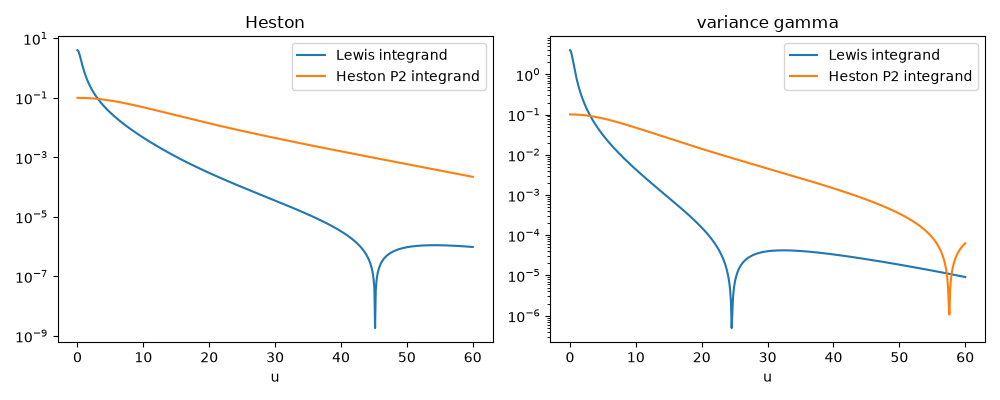
Heston: Lewis 0.41986248, Heston's formula 0.41986248
variance gamma: Lewis 0.73063766, Heston's formula 0.73063765

import matplotlib.pyplot as plt
import numpy as np

from financialkit.stochastic_volatility import HestonModel, VarianceGammaModel, heston_price, lewis_price

S, K, T, r = 100.0, 110.0, 0.25, 0.0
models = {"Heston": HestonModel(0.04, 1.5, 0.04, 0.5, -0.7), "variance gamma": VarianceGammaModel(0.2, 0.2, -0.2)}

fig, axes = plt.subplots(1, 2, figsize=(10, 4))
u = np.linspace(1e-3, 60, 600)
kap = np.log(S / K)
for ax, (name, m) in zip(axes, models.items(), strict=True):
    lewis = np.real(np.exp(1j * u * kap) * m.char_func(u - 0.5j, T)) / (u**2 + 0.25)
    p2 = np.real(np.exp(1j * u * kap) * m.char_func(u, T) / (1j * u))
    ax.plot(u, np.abs(lewis), label="Lewis integrand")
    ax.plot(u, np.abs(p2), label="Heston P2 integrand")
    ax.set_yscale("log")
    ax.set_xlabel("u")
    ax.set_title(name)
    ax.legend()
    print(f"{name}: Lewis {lewis_price(m, S, K, T, r):.8f}, Heston's formula {heston_price(m, S, K, T, r):.8f}")
fig.tight_layout()

plt.show()