Fama-MacBeth regressions

Eugene Fama and James MacBeth (1973) estimated risk premia with a cross-sectional regression each month,

\[r^e_{it} = \gamma_{0t} + \gamma_{1t}\,\beta_i + \gamma_{2t}\,\beta_i^2 + \gamma_{3t}\,s_i + u_{it},\]

and averaged the slopes over time, taking standard errors from the month-to-month variation of the slopes, which automatically accounts for the correlation of returns across stocks. If the CAPM holds, the average \(\gamma_1\) is the market premium, while \(\beta^2\) and residual risk \(s_i\) earn nothing.

import matplotlib.pyplot as plt
import numpy as np

from financialkit.asset_pricing import fama_macbeth, simulate_factor_model, time_series_regression
from financialkit.asset_pricing.visualizers import plot_fama_macbeth

rng = np.random.default_rng(1973)
N, T, premium = 100, 600, 0.006
betas = np.linspace(0.4, 1.8, N)
idio = rng.uniform(0.03, 0.10, N)
panel = simulate_factor_model(T, betas, [premium], [[0.0020]], idio_vol=idio, rng=rng)

# Betas from first-pass time-series regressions, then monthly cross-sections.
fm = fama_macbeth(panel.excess_returns, factors=panel.factors)
# For a traded factor the slope estimates the factor's realised mean
# return, which itself differs from the 0.6% premium by sampling error.
realised = panel.factors.mean()
print(f"market premium: {fm.premia[1]:.5f} (se {fm.std_errors[1]:.5f}); realised factor mean {realised:.5f}")

fig, ax = plt.subplots(figsize=(8, 3.5))
plot_fama_macbeth(fm, index=1, ax=ax, true_value=realised)
ax.set_title("monthly slope on beta, against the factor's realised mean")
fig.tight_layout()

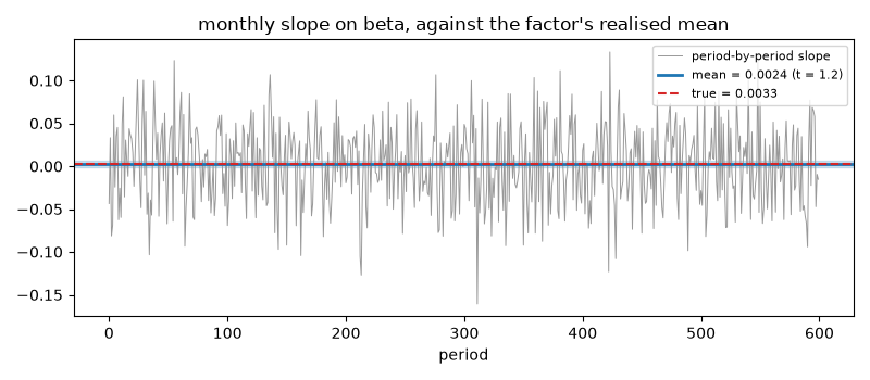
market premium: 0.00236 (se 0.00191); realised factor mean 0.00326

Fama and MacBeth’s test of the CAPM

Adding beta squared and residual risk as regressors: neither should be priced. (Beta and its square are nearly collinear, so the individual slopes are imprecise.)

ts = time_series_regression(panel.excess_returns, panel.factors)
b = ts.betas[:, 0]
s = ts.residuals.std(axis=0)
fm3 = fama_macbeth(panel.excess_returns, betas=np.column_stack([b, b**2, s]))
for name, g, t in zip(["gamma_0", "beta", "beta^2", "resid. sd"], fm3.premia, fm3.t_values, strict=True):
    print(f"{name:>9}: {g:+.5f}  (t = {t:+.2f})")

  gamma_0: +0.00355  (t = +1.61)
     beta: -0.00266  (t = -0.61)
   beta^2: +0.00225  (t = +1.25)
resid. sd: -0.00154  (t = -0.10)

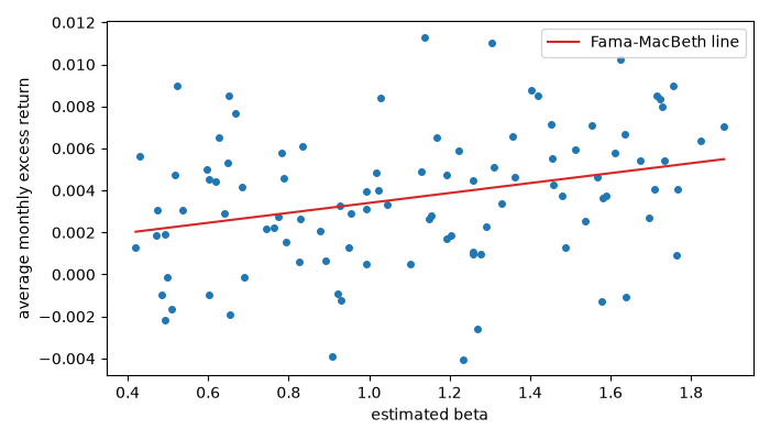
Average returns against beta

fig, ax = plt.subplots(figsize=(7, 4))
ax.plot(b, panel.excess_returns.mean(axis=0), "o", ms=4)
bb = np.linspace(b.min(), b.max(), 2)
ax.plot(bb, fm.premia[0] + fm.premia[1] * bb, "C3", label="Fama-MacBeth line")
ax.legend()
ax.set_xlabel("estimated beta")
ax.set_ylabel("average monthly excess return")
fig.tight_layout()

plt.show()