Vasicek’s large homogeneous portfolio

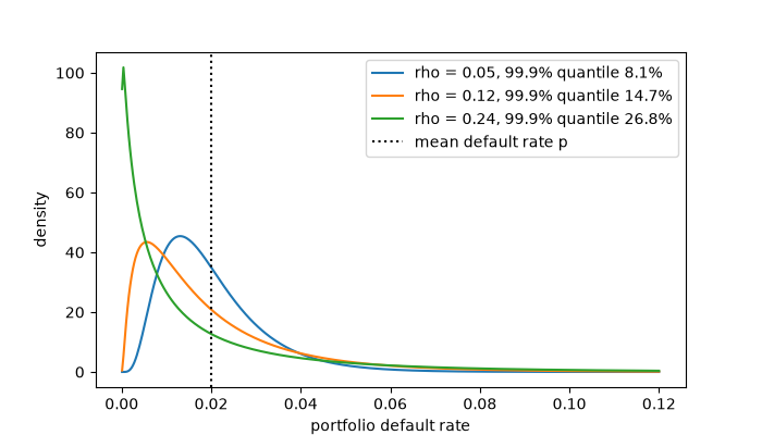
Vasicek (1987) let every loan default when its asset return \(\sqrt\rho M + \sqrt{1-\rho}\,\varepsilon_i\) falls below \(N^{-1}(p)\). Given the common factor \(M\), defaults are independent, so in a large pool the default rate is the deterministic \(p(M)\), and its distribution is known in closed form. Correlation does not change the expected loss, only how it is spread out: at high correlation most years are quiet and a few are disasters.

import matplotlib.pyplot as plt
import numpy as np

from financialkit.credit import simulate_one_factor_defaults, vasicek_cdf, vasicek_pdf, vasicek_quantile

p = 0.02
x = np.linspace(1e-4, 0.12, 400)
fig, ax = plt.subplots(figsize=(7, 4))
for rho in (0.05, 0.12, 0.24):
    ax.plot(x, vasicek_pdf(x, p, rho), label=f"rho = {rho}, 99.9% quantile {vasicek_quantile(0.999, p, rho):.1%}")
ax.axvline(p, color="k", ls=":", label="mean default rate p")
ax.set_xlabel("portfolio default rate")
ax.set_ylabel("density")
ax.legend()

<matplotlib.legend.Legend object at 0x11659a660>

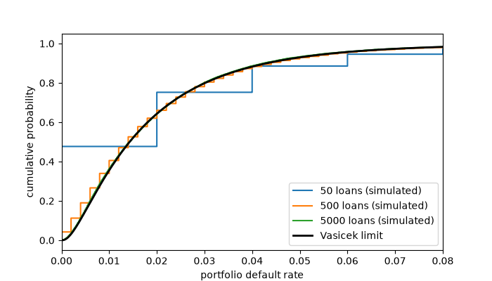
Finite pools converge to the limit

rho = 0.12
fig, ax = plt.subplots(figsize=(7, 4))
for n in (50, 500, 5000):
    frac = np.sort(simulate_one_factor_defaults(p, rho, n, 20000, rng=0) / n)
    ax.step(frac, np.arange(1, frac.size + 1) / frac.size, where="post", label=f"{n} loans (simulated)")
ax.plot(x, vasicek_cdf(x, p, rho), "k", lw=2, label="Vasicek limit")
ax.set_xlim(0, 0.08)
ax.set_xlabel("portfolio default rate")
ax.set_ylabel("cumulative probability")
ax.legend()

plt.show()