Hull and White: pricing CDO tranches without Monte Carlo

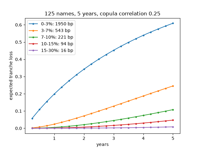
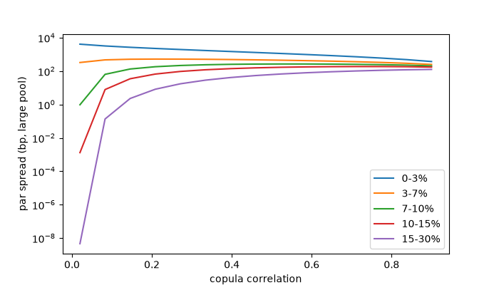
A tranche of a synthetic CDO absorbs portfolio losses between its attachment and detachment points. Hull and White (2004) priced tranches in Li’s one-factor Gaussian copula by conditioning on the common factor: given it, defaults are independent and the pool loss is binomial, so the expected tranche loss at each date is one integral over the factor. Raising the correlation moves risk from the equity tranche, which loses less, to the senior tranches, which lose more.

import matplotlib.pyplot as plt
import numpy as np

from financialkit.credit import HazardCurve, expected_tranche_loss, tranche_spread
from financialkit.credit.visualizers import plot_tranche_losses

curve = HazardCurve.flat(0.012)
tranches = [(0.0, 0.03), (0.03, 0.07), (0.07, 0.10), (0.10, 0.15), (0.15, 0.30)]
res = [tranche_spread(a, d, curve, 0.25, 5.0, 0.03, n_names=125) for a, d in tranches]
ax = plot_tranche_losses(res)
ax.set_title("125 names, 5 years, copula correlation 0.25")

Text(0.5, 1.0, '125 names, 5 years, copula correlation 0.25')

Spreads against correlation

rhos = np.linspace(0.02, 0.9, 15)
fig, ax = plt.subplots(figsize=(7, 4))
for a, d in tranches:
    s = [tranche_spread(a, d, curve, rho, 5.0, 0.03).par_spread for rho in rhos]
    ax.semilogy(rhos, 1e4 * np.array(s), label=f"{100 * a:g}-{100 * d:g}%")
ax.set_xlabel("copula correlation")
ax.set_ylabel("par spread (bp, large pool)")
ax.legend()

<matplotlib.legend.Legend object at 0x1163b38c0>

Finite pool versus the large-pool limit

p = float(curve.default_probability(5.0))
for n in (25, 125, 1000, None):
    el = expected_tranche_loss(0.03, 0.07, p, 0.25, n_names=n)
    print(f"{'LHP' if n is None else n:>5}: expected 3-7% tranche loss at 5y = {el:.4f}")

plt.show()

  25: expected 3-7% tranche loss at 5y = 0.2634
 125: expected 3-7% tranche loss at 5y = 0.2454
1000: expected 3-7% tranche loss at 5y = 0.2409
 LHP: expected 3-7% tranche loss at 5y = 0.2398