CreditRisk+ and Panjer’s recursion

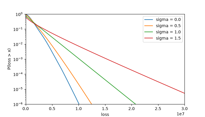
Credit Suisse First Boston’s CreditRisk+ (1997) treated defaults like insurance claims: Poisson events with rates driven by a gamma-distributed sector factor, and exposures rounded to multiples of a loss unit. The default count is then negative binomial, and Panjer’s (1981) recursion produces the whole loss distribution exactly, without simulation. The factor’s volatility \(\sigma\) fattens the tail without changing the expected loss.

import matplotlib.pyplot as plt
import numpy as np

from financialkit.credit import creditrisk_plus
from financialkit.credit.visualizers import plot_loss_distribution

rng = np.random.default_rng(0)
exposures = np.round(rng.lognormal(np.log(2e5), 0.9, 300), -4)
pds = np.clip(rng.lognormal(np.log(0.01), 0.8, 300), 1e-4, 0.2)
unit = 50_000.0

fig, ax = plt.subplots(1, 2, figsize=(12, 4))
for a, sigma in zip(ax, (0.0, 1.0), strict=True):
    dist = creditrisk_plus(exposures, pds, sigma=sigma, unit=unit)
    plot_loss_distribution(dist, alpha=0.999, ax=a, log=True)
    a.set_title(f"sector volatility sigma = {sigma}")
    a.set_xlim(0, 2.5e7)
    a.set_ylim(1e-8, 1)
    print(f"sigma = {sigma}: EL {dist.mean:,.0f}, sd {dist.std:,.0f}, 99.9% UL {dist.unexpected_loss(0.999):,.0f}")

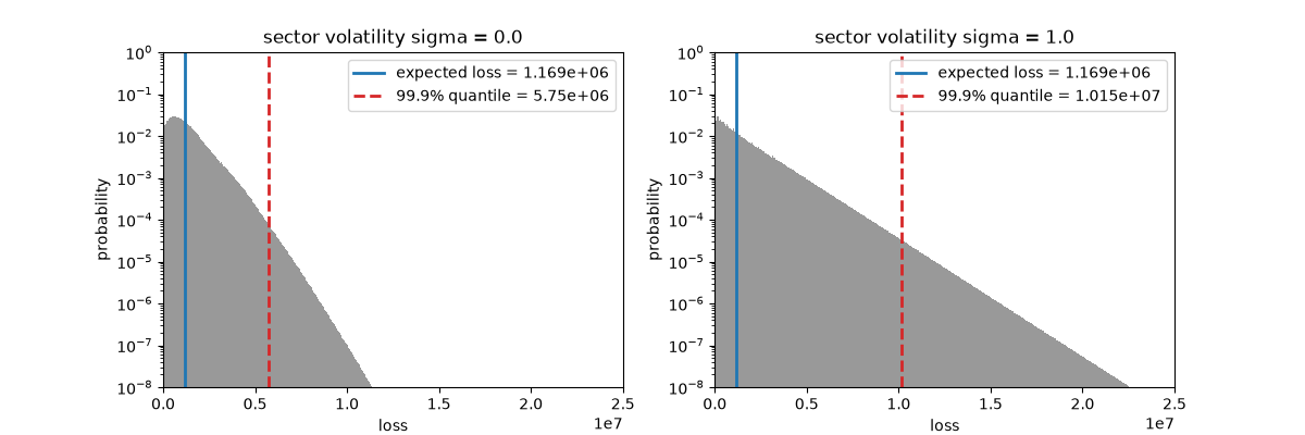
sigma = 0.0: EL 1,168,615, sd 892,123, 99.9% UL 4,581,385
sigma = 1.0: EL 1,168,614, sd 1,470,212, 99.9% UL 8,981,386

Tail probabilities

fig, ax = plt.subplots(figsize=(7, 4))
for sigma in (0.0, 0.5, 1.0, 1.5):
    d = creditrisk_plus(exposures, pds, sigma=sigma, unit=unit)
    ax.semilogy(d.losses, 1 - np.cumsum(d.pmf), label=f"sigma = {sigma}")
ax.set_xlim(0, 3e7)
ax.set_ylim(1e-6, 1)
ax.set_xlabel("loss")
ax.set_ylabel("P(loss > x)")
ax.legend()

plt.show()