Li’s Gaussian copula for default times

Li (2000) took each name’s default-time distribution from its CDS curve and joined them with a Gaussian copula: correlated normals become uniforms, and each uniform is mapped through that name’s survival curve. The marginals stay exactly as the market implies; the copula correlation controls how often names default together, which is what a first-to-default basket or a CDO tranche is really priced on.

import matplotlib.pyplot as plt
import numpy as np

from financialkit.credit import HazardCurve, copula_default_times, default_correlation, joint_default_probability, nth_to_default_probability

curve = HazardCurve.flat(0.02)
T = 5.0
p = float(curve.default_probability(T))

fig, ax = plt.subplots(1, 2, figsize=(11, 4.5))
for a, rho in zip(ax, (0.0, 0.7), strict=True):
    tau = copula_default_times(curve, rho, 3000, n_names=2, rng=0)
    a.scatter(np.minimum(tau[:, 0], 60), np.minimum(tau[:, 1], 60), s=3, alpha=0.4)
    a.axvline(T, color="C3", lw=0.8)
    a.axhline(T, color="C3", lw=0.8)
    a.set_xlim(0, 60)
    a.set_ylim(0, 60)
    a.set_title(f"rho = {rho}: P(both by {T:g}y) = {joint_default_probability(p, p, rho):.4f}")
    a.set_xlabel("default time, name 1")
ax[0].set_ylabel("default time, name 2")

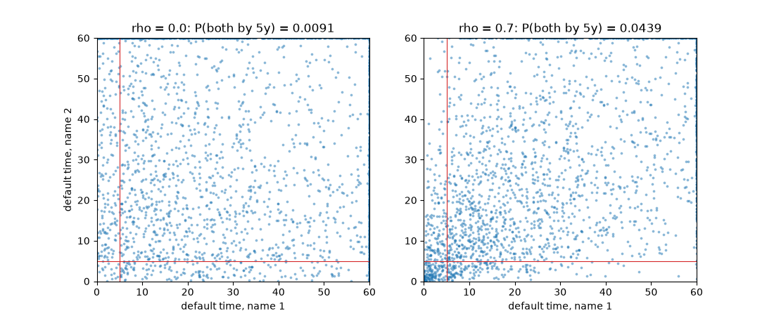
Text(104.22222222222221, 0.5, 'default time, name 2')

Default correlation is much smaller than copula correlation

rhos = np.linspace(0, 0.95, 20)
print("copula rho -> default-indicator correlation:", [f"{r:.2f}->{default_correlation(p, p, r):.3f}" for r in rhos[::5]])

copula rho -> default-indicator correlation: ['0.00->-0.000', '0.25->0.102', '0.50->0.246', '0.75->0.455']

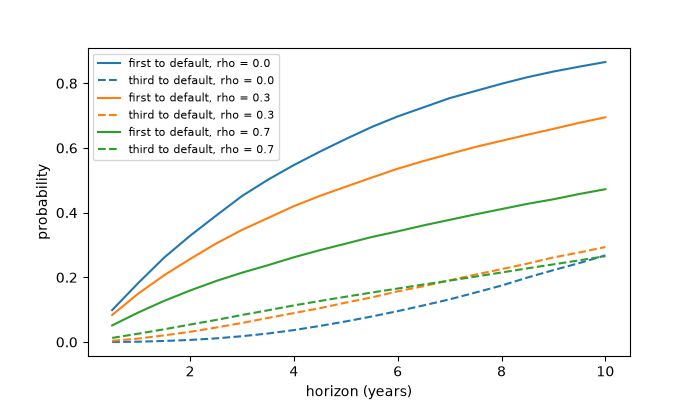
A ten-name basket

horizons = np.linspace(0.5, 10, 20)
fig, ax = plt.subplots(figsize=(7, 4))
for rho in (0.0, 0.3, 0.7):
    tau = copula_default_times(curve, rho, 20000, n_names=10, rng=1)
    ax.plot(horizons, nth_to_default_probability(tau, 1, horizons), label=f"first to default, rho = {rho}")
    ax.plot(horizons, nth_to_default_probability(tau, 3, horizons), ls="--", color=ax.lines[-1].get_color(), label=f"third to default, rho = {rho}")
ax.set_xlabel("horizon (years)")
ax.set_ylabel("probability")
ax.legend(fontsize=8)

plt.show()