Merton’s analytic frontier

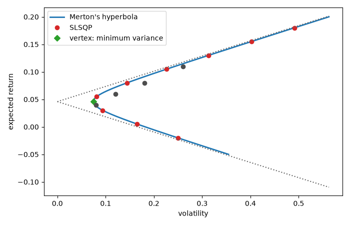
Robert Merton (1972) derived the unconstrained frontier in closed form. Four scalars,

\[A = \mathbf 1'\Sigma^{-1}\mu,\quad B = \mu'\Sigma^{-1}\mu,\quad C = \mathbf 1'\Sigma^{-1}\mathbf 1,\quad D = BC - A^2,\]

give the least variance at every mean, \(\sigma^2(m) = (Cm^2 - 2Am + B)/D\): a hyperbola with vertex at the minimum-variance portfolio \((1/\sqrt C, A/C)\) and asymptotes of slope \(\pm\sqrt{D/C}\). Every frontier portfolio is a mix of two of them (two-fund separation).

import matplotlib.pyplot as plt
import numpy as np

from financialkit.portfolio import efficient_portfolio, frontier_constants
from financialkit.portfolio.utils import solve_qp

mu = np.array([0.04, 0.06, 0.08, 0.11])
vol = np.array([0.08, 0.12, 0.18, 0.26])
corr = np.array([[1.0, 0.3, 0.2, 0.1], [0.3, 1.0, 0.5, 0.4], [0.2, 0.5, 1.0, 0.6], [0.1, 0.4, 0.6, 1.0]])
cov = corr * np.outer(vol, vol)
fc = frontier_constants(mu, cov)
print(f"A = {fc.A:.3f}, B = {fc.B:.4f}, C = {fc.C:.2f}, D = {fc.D:.4f}")

A = 8.271, B = 0.4556, C = 180.40, D = 13.7838

Closed form against a numerical optimizer

m = np.linspace(-0.05, 0.2, 200)
fig, ax = plt.subplots(figsize=(7, 4.5))
ax.plot(fc.volatility(m), m, lw=2, label="Merton's hyperbola")
targets = np.linspace(-0.02, 0.18, 9)
numeric = [np.sqrt(w @ cov @ w) for w in (solve_qp(cov, np.vstack([np.ones(4), mu]), [1.0, t], bounds=(-10.0, 10.0)) for t in targets)]
ax.plot(numeric, targets, "o", color="C3", label="SLSQP")
s = np.linspace(0, fc.volatility(0.2), 2)
for sign in (1, -1):
    ax.plot(s, fc.gmv_return + sign * fc.asymptote_slope() * s, ":", color="0.4")
ax.plot(fc.gmv_volatility, fc.gmv_return, "D", color="C2", label="vertex: minimum variance")
ax.plot(vol, mu, "o", color="0.3")
ax.set_xlabel("volatility")
ax.set_ylabel("expected return")
ax.legend()
fig.tight_layout()

Two-fund separation

The weights are linear in the target mean, so any two frontier portfolios span the whole frontier.

w1, w2 = efficient_portfolio(mu, cov, 0.05).weights, efficient_portfolio(mu, cov, 0.10).weights
w3 = efficient_portfolio(mu, cov, 0.15).weights
print("w(15%) = 2 w(10%) - w(5%):", np.allclose(w3, 2 * w2 - w1))
plt.show()

w(15%) = 2 w(10%) - w(5%): True