DeMiguel-Garlappi-Uppal: optimal versus 1/N

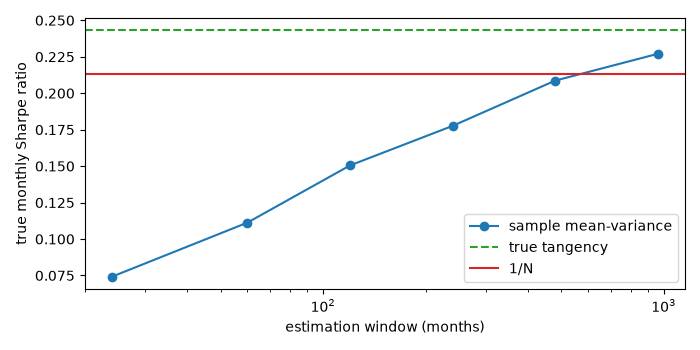
DeMiguel, Garlappi and Uppal (2009) re-estimated fourteen optimized portfolio rules on rolling windows and compared their out-of-sample Sharpe ratios with simply holding every asset equally. None beat 1/N reliably. Here the true model is known: ten assets with a genuinely better tangency portfolio. The sample mean-variance rule, the tangency portfolio of the estimated moments, still loses to 1/N unless its estimation window is very long, because errors in the estimated means swamp the gain from optimizing.

import matplotlib.pyplot as plt
import numpy as np

from financialkit.portfolio import equal_weight, min_variance_portfolio, out_of_sample_returns, tangency_portfolio, two_fund_allocation
from financialkit.portfolio.visualizers import plot_out_of_sample

rng = np.random.default_rng(4)
d = 10
mu = np.linspace(0.006, 0.010, d)
vol = np.linspace(0.03, 0.08, d)
corr = 0.4 + 0.6 * np.eye(d)
cov = corr * np.outer(vol, vol)
true_t = tangency_portfolio(mu, cov)
ew = equal_weight(d)
print(f"true monthly Sharpe: tangency {true_t.sharpe_ratio():.3f}, 1/N {ew @ mu / np.sqrt(ew @ cov @ ew):.3f}")

R = rng.multivariate_normal(mu, cov, size=600)


def sample_mean_variance(past):
    # Sigma^-1 mu scaled to unit gross exposure: the sample tangency direction,
    # well defined even when the estimated minimum-variance mean is negative.
    w = two_fund_allocation(past.mean(axis=0), np.cov(past, rowvar=False), 0.0, 1.0).weights
    return w / np.abs(w).sum()


def sample_min_variance(past):
    return min_variance_portfolio(np.cov(past, rowvar=False), long_only=True).weights

true monthly Sharpe: tangency 0.243, 1/N 0.213

Out of sample with a 60-month window

results = [
    out_of_sample_returns(R, lambda past: ew, 60, "1/N"),
    out_of_sample_returns(R, sample_mean_variance, 60, "sample mean-variance"),
    out_of_sample_returns(R, sample_min_variance, 60, "long-only min variance"),
]
plot_out_of_sample(results)
for res in results:
    print(f"{res.name:>24}: Sharpe {res.sharpe:.3f}, turnover {res.turnover:.2f}")

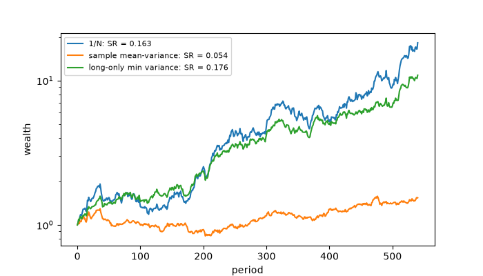
                   1/N: Sharpe 0.163, turnover 0.00
  sample mean-variance: Sharpe 0.054, turnover 0.20
long-only min variance: Sharpe 0.176, turnover 0.06

How long a window does optimization need?

The true Sharpe ratio of the sample mean-variance rule, averaged over histories, approaches the optimum only slowly as the window grows. Each point evaluates the estimated weights under the true moments.

windows = [24, 60, 120, 240, 480, 960]
sr_est = []
for T in windows:
    vals = []
    for _ in range(40):
        X = rng.multivariate_normal(mu, cov, size=T)
        w = sample_mean_variance(X)
        vals.append(w @ mu / np.sqrt(w @ cov @ w))
    sr_est.append(np.mean(vals))
fig, ax = plt.subplots(figsize=(7, 3.5))
ax.semilogx(windows, sr_est, "o-", label="sample mean-variance")
ax.axhline(true_t.sharpe_ratio(), color="C2", ls="--", label="true tangency")
ax.axhline(ew @ mu / np.sqrt(ew @ cov @ ew), color="C3", label="1/N")
ax.set_xlabel("estimation window (months)")
ax.set_ylabel("true monthly Sharpe ratio")
ax.legend()
fig.tight_layout()
plt.show()