Rockafellar-Uryasev CVaR optimization

Value at risk is not convex in the portfolio weights, so minimizing it is hard. R. Tyrrell Rockafellar and Stanislav Uryasev (2000) showed that conditional value at risk (expected shortfall) is, and better: over a set of scenarios, minimizing it is a linear program,

\[\min_{w,\zeta,u}\; \zeta + \frac{1}{(1-\alpha)n}\sum_k u_k \quad\text{s.t.}\quad u_k \ge -r_k'w - \zeta,\; u_k \ge 0,\]

and the optimal \(\zeta\) is the VaR as a by-product. With fat-tailed, skewed scenarios, the CVaR-optimal portfolio avoids the asset whose variance looks modest but whose crashes are large.

import matplotlib.pyplot as plt
import numpy as np

from financialkit.portfolio import cvar_optimization, efficient_portfolio
from financialkit.portfolio.visualizers import plot_weights
from financialkit.risk import expected_shortfall

rng = np.random.default_rng(9)
names = ["bonds", "equity", "credit carry", "commodities"]
n = 2000
R = rng.multivariate_normal([0.003, 0.006, 0.0, 0.005], np.diag([0.01, 0.045, 0.008, 0.05]) ** 2, size=n)
# The carry trade earns a steady premium but loses heavily in crash months, alongside equities.
crash = rng.random(n) < 0.04
R[:, 2] += np.where(crash, -0.10, 0.009)
R[:, 1] += np.where(crash, -0.05, 0.0)

Minimum-CVaR versus minimum-variance at the same mean

target = 0.004
cv = cvar_optimization(R, 0.95, target_return=target)
mv = efficient_portfolio(R.mean(axis=0), np.cov(R, rowvar=False), target, long_only=True)
fig, axes = plt.subplots(1, 2, figsize=(10, 3.5), sharey=True)
plot_weights(mv.weights, names, ax=axes[0]).set_title("minimum variance")
plot_weights(cv.weights, names, ax=axes[1]).set_title("minimum 95% CVaR")
fig.tight_layout()
for label, w in [("min variance", mv.weights), ("min CVaR", cv.weights)]:
    pnl = R @ w
    print(f"{label:>12}: vol {pnl.std():.4f}, 95% ES {expected_shortfall(pnl, 0.95):.4f}")
print(f"LP: CVaR {cv.cvar:.4f}, VaR (zeta) {cv.var:.4f}")

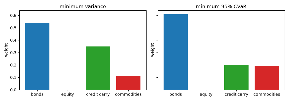
min variance: vol 0.0111, 95% ES 0.0291
    min CVaR: vol 0.0124, 95% ES 0.0226
LP: CVaR 0.0226, VaR (zeta) 0.0170

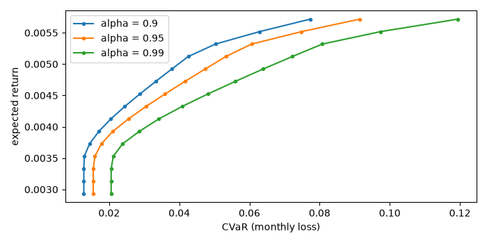
The mean-CVaR frontier

targets = np.linspace(R.mean(axis=0).min() + 1e-4, R.mean(axis=0).max() - 1e-4, 15)
fig, ax = plt.subplots(figsize=(7, 3.5))
for a in [0.9, 0.95, 0.99]:
    ax.plot([cvar_optimization(R, a, t).cvar for t in targets], targets, "o-", ms=3, label=f"alpha = {a}")
ax.set_xlabel("CVaR (monthly loss)")
ax.set_ylabel("expected return")
ax.legend()
fig.tight_layout()
plt.show()