Lopez de Prado’s hierarchical risk parity

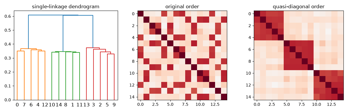
Marcos Lopez de Prado (2016) observed that inverting a noisy covariance matrix, as every quadratic optimizer does, amplifies its errors. His hierarchical risk parity never inverts it: it clusters assets by the correlation distance \(\sqrt{(1-\rho_{ij})/2}\), reorders them along the dendrogram so similar assets sit together, then splits capital top down between halves in inverse proportion to their variance. Its risk varies less from one estimation sample to the next than the minimum-variance portfolio’s, though with few observations per asset minimum variance can still be less risky on average.

import matplotlib.pyplot as plt
import numpy as np
from scipy.cluster.hierarchy import dendrogram

from financialkit.portfolio import hierarchical_risk_parity, min_variance_portfolio

rng = np.random.default_rng(10)
# Three hidden clusters of correlated assets.
d, k = 15, 3
labels = np.repeat(np.arange(k), d // k)
corr = np.where(labels[:, None] == labels[None, :], 0.7, 0.15)
np.fill_diagonal(corr, 1.0)
perm = rng.permutation(d)
corr = corr[np.ix_(perm, perm)]
vol = rng.uniform(0.1, 0.3, d)
cov = corr * np.outer(vol, vol)
L = np.linalg.cholesky(cov)

The dendrogram and the quasi-diagonalized correlation matrix

X = rng.standard_normal((120, d)) @ L.T
S = np.cov(X, rowvar=False)
hrp = hierarchical_risk_parity(S)
fig, (ax1, ax2, ax3) = plt.subplots(1, 3, figsize=(12, 3.8))
dendrogram(hrp.linkage, ax=ax1, color_threshold=0.5)
ax1.set_title("single-linkage dendrogram")
ax2.imshow(np.corrcoef(X, rowvar=False), cmap="RdBu_r", vmin=-1, vmax=1)
ax2.set_title("original order")
ax3.imshow(np.corrcoef(X, rowvar=False)[np.ix_(hrp.order, hrp.order)], cmap="RdBu_r", vmin=-1, vmax=1)
ax3.set_title("quasi-diagonal order")
fig.tight_layout()

Stability out of sample

Re-estimate on 100 fresh samples of 60 observations and compare each portfolio’s true volatility: HRP’s spread is the narrower one.

vols = {"HRP": [], "minimum variance": [], "1/N": []}
for _ in range(100):
    X = rng.standard_normal((60, d)) @ L.T
    S = np.cov(X, rowvar=False)
    for name, w in [("HRP", hierarchical_risk_parity(S).weights), ("minimum variance", min_variance_portfolio(S).weights), ("1/N", np.full(d, 1 / d))]:
        vols[name].append(np.sqrt(w @ cov @ w))
fig, ax = plt.subplots(figsize=(7, 3.5))
ax.boxplot(list(vols.values()), tick_labels=list(vols))
ax.axhline(min_variance_portfolio(cov).volatility, color="C2", ls="--", label="true minimum variance")
ax.set_ylabel("true volatility")
ax.legend()
fig.tight_layout()
for name, v in vols.items():
    print(f"{name:>16}: mean vol {np.mean(v):.3f}, spread {np.std(v):.3f}")
plt.show()

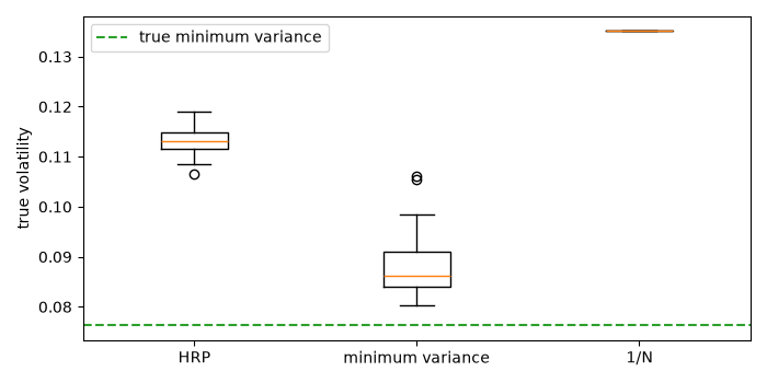
             HRP: mean vol 0.113, spread 0.002
minimum variance: mean vol 0.088, spread 0.005
             1/N: mean vol 0.135, spread 0.000