Fama’s runs test

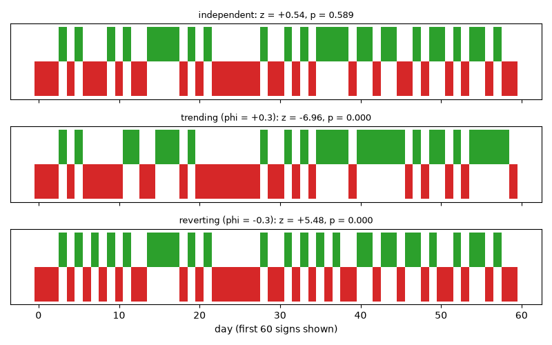
Correlation coefficients can be dominated by a few large changes. In his 1965 thesis Eugene Fama added a distribution-free check on the 30 Dow Jones stocks: count the runs, the unbroken sequences of price changes with the same sign. Positive dependence produces long runs and too few of them; reversals produce too many. Under independence the number of runs is approximately normal with a known mean and variance, and Fama found the observed counts close to the expected ones.

import matplotlib.pyplot as plt
import numpy as np
from scipy.signal import lfilter

from financialkit.time_series import runs_test

Runs in three series

Independent changes, positively autocorrelated changes (trends), and negatively autocorrelated changes (reversals, such as bid-ask bounce).

rng = np.random.default_rng(1965)
e = rng.standard_normal(1000)
cases = {
    "independent": e,
    "trending (phi = +0.3)": lfilter([1.0], [1.0, -0.3], e),
    "reverting (phi = -0.3)": lfilter([1.0], [1.0, 0.3], e),
}

fig, axes = plt.subplots(3, 1, figsize=(8, 5), sharex=True)
for ax, (name, x) in zip(axes, cases.items(), strict=True):
    res = runs_test(x)
    ax.bar(np.arange(60), np.sign(x[:60]), color=np.where(x[:60] > 0, "C2", "C3"), width=1.0)
    ax.set_yticks([])
    ax.set_title(f"{name}: z = {res.statistic:+.2f}, p = {res.pvalue:.3f}", fontsize=9)
axes[-1].set_xlabel("day (first 60 signs shown)")
fig.tight_layout()

The test’s size

Under independence the statistic is close to standard normal, so the test rejects about 5% of the time.

z = np.array([runs_test(rng.standard_normal(250)).statistic for _ in range(1000)])
fig, ax = plt.subplots()
ax.hist(z, bins=30, density=True, color="0.7", label="1000 independent samples")
grid = np.linspace(-4, 4, 200)
ax.plot(grid, np.exp(-(grid**2) / 2) / np.sqrt(2 * np.pi), "k", label="N(0, 1)")
ax.set_xlabel("runs statistic")
ax.legend()
print(f"rejection rate at 5%: {np.mean(np.abs(z) > 1.96):.3f}")
plt.show()

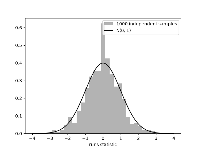
rejection rate at 5%: 0.051