Lo-MacKinlay variance ratio

If log prices follow a random walk, the variance of \(q\)-week returns is \(q\) times that of one-week returns. Andrew Lo and Craig MacKinlay (1988) turned this into a test,

\[VR(q) = \frac{\operatorname{Var}(r_t + \dots + r_{t-q+1})}{q\operatorname{Var}(r_t)} \approx 1 + 2\sum_{k=1}^{q-1}\Bigl(1 - \frac kq\Bigr)\rho_k,\]

with a heteroskedasticity-consistent standard error so that volatility clustering alone cannot cause a rejection. Weekly returns on U.S. stock indices from 1962 to 1985 gave \(VR(2) \approx 1.3\), strongly rejecting the random walk, mostly through the positive autocorrelation of small-stock portfolios.

import matplotlib.pyplot as plt
import numpy as np
from scipy.signal import lfilter

from financialkit.time_series import GJRGARCH, variance_ratio
from financialkit.time_series.visualizers import plot_variance_ratio

A random walk and an index with autocorrelated returns

Twenty-four years of weekly returns. The second series has first-order autocorrelation 0.3, like Lo and MacKinlay’s equal-weighted index.

rng = np.random.default_rng(1988)
T = 1216
e = 0.02 * rng.standard_normal(T)
walk = np.r_[0.0, np.cumsum(e)]
index = np.r_[0.0, np.cumsum(lfilter([1.0], [1.0, -0.3], e))]
qs = [2, 4, 8, 16]

fig, ax = plt.subplots()
for name, p in (("random walk", walk), ("AR(1) returns, phi = 0.3", index)):
    res = variance_ratio(p, q=qs)
    plot_variance_ratio(res, ax=ax, label=name)
    print(f"{name}: VR = {res.ratio.round(2)}, z* = {res.z_robust.round(1)}")
ax.set_title("Variance ratios with the 95% random-walk band")

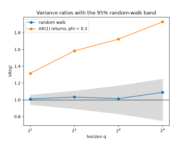
random walk: VR = [1.01 1.03 1.01 1.09], z* = [0.3 0.6 0.2 0.7]
AR(1) returns, phi = 0.3: VR = [1.31 1.58 1.72 1.93], z* = [10.2 10.3  8.1  7.1]

Text(0.5, 1.0, 'Variance ratios with the 95% random-walk band')

Robustness to volatility clustering

Under GJR-GARCH increments the random walk holds, but the homoskedastic \(z(2)\) is too dispersed; the robust \(z^*(2)\) stays close to standard normal.

m = GJRGARCH(omega=0.02, alpha=0.05, gamma=0.15, beta=0.85)
z, zr = [], []
for _ in range(300):
    res = variance_ratio(np.cumsum(m.simulate(1000, burn=200, rng=rng).returns), q=2)
    z.append(res.z[0])
    zr.append(res.z_robust[0])
fig, ax = plt.subplots()
ax.hist([z, zr], bins=25, density=True, histtype="step", lw=1.5, label=["z (homoskedastic)", "z* (robust)"])
g = np.linspace(-5, 5, 200)
ax.plot(g, np.exp(-(g**2) / 2) / np.sqrt(2 * np.pi), "k", label="N(0, 1)")
ax.set_xlabel("statistic under the null")
ax.legend()
print(f"rejection rate at 5%: z {np.mean(np.abs(z) > 1.96):.2f}, z* {np.mean(np.abs(zr) > 1.96):.2f}")
plt.show()

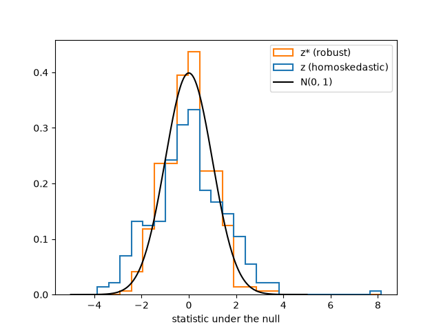
rejection rate at 5%: z 0.20, z* 0.04