Scale-free networks: preferential attachment (Barabási and Albert 1999)

Real networks, from the Web to peer-to-peer overlays, have a few huge hubs and many small nodes: their degree distribution follows a power law, unlike the narrow distribution of a random graph. Barabási and Albert explained it with growth plus preferential attachment: newcomers link to existing nodes with probability proportional to their degree, so the rich get richer.

What to look for

On log-log axes the degree distribution is close to a straight line of slope -3, and the largest degree is several times what a random graph of the same density reaches. Hubs make gossip fast, but they are also a weak point: removing 5% of the nodes at random leaves the network in one piece, while removing the 5% largest hubs already cuts a tenth of the peers off.

The history behind this experiment: Breakthroughs in Peer-to-Peer Networking.

Degree distributions

import collections

import matplotlib.pyplot as plt
import numpy as np

import blockchainkit as bk

n = 3000
scale_free = bk.network.barabasi_albert(n, 2, seed=1)
random_graph = bk.network.erdos_renyi(n, 4 / (n - 1), seed=1)
print("largest degree:", max(scale_free.degrees()), "vs", max(random_graph.degrees()))
assert max(scale_free.degrees()) > 4 * max(random_graph.degrees())

counts = collections.Counter(scale_free.degrees())
degrees = np.array(sorted(counts))
share = np.array([counts[d] for d in degrees]) / n
fit = degrees <= 30  # Fit where every degree is still well sampled.
coefficients = np.polyfit(np.log(degrees[fit]), np.log(share[fit]), 1)
slope = coefficients[0]
print(f"fitted exponent {slope:.2f}")
assert -3.5 < slope < -2.3

largest degree: 129 vs 13
fitted exponent -2.76

Targeted attacks hurt

Remove 5% of the nodes, either the largest hubs or a random choice.

def largest_component_after_removing(graph, removed):
    kept = [u for u in range(graph.n) if u not in removed]
    index = {u: i for i, u in enumerate(kept)}
    edges = [(index[u], index[v]) for u, v in graph.edges if u in index and v in index]
    return len(bk.network.Graph(len(kept), edges).components()[0]) / len(kept)


hubs = set(sorted(range(n), key=lambda u: -scale_free.degrees()[u])[: n // 20])
rng = np.random.default_rng(0)
randoms = set(rng.choice(n, n // 20, replace=False).tolist())
targeted = largest_component_after_removing(scale_free, hubs)
failures = largest_component_after_removing(scale_free, randoms)
print(f"largest component: {failures:.2f} after random failures, {targeted:.2f} after attack")
assert failures > 0.99 and targeted < 0.95

fig, (left, right) = plt.subplots(1, 2, figsize=(10, 4))
left.loglog(degrees, share, "o", markersize=4, label="Barabási-Albert")
er = collections.Counter(random_graph.degrees())
left.loglog(sorted(er), [er[d] / n for d in sorted(er)], "s", markersize=4, label="Erdős-Rényi")
left.loglog(degrees[fit], np.exp(np.polyval(coefficients, np.log(degrees[fit]))), color="black")
left.set(xlabel="degree k", ylabel="P(k)", title="Power law versus Poisson")
left.legend()
right.bar(["random 5%", "top-hub 5%"], [failures, targeted], color=["#16a34a", "#dc2626"])
right.set(ylabel="largest component share", title="Robust, yet fragile")
fig.tight_layout()

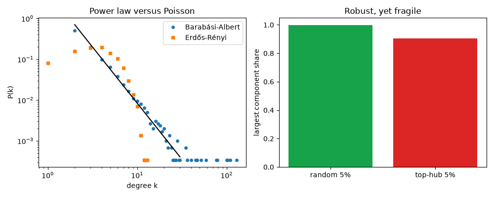
largest component: 1.00 after random failures, 0.90 after attack

Exercise

Compute the average path length of both graphs on 500 nodes. Which is shorter, and what role do the hubs play?