Kyle’s insider and the price impact lambda

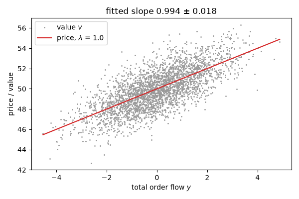
Albert Kyle (1985) placed an insider who knows the liquidation value \(v \sim N(p_0, \sigma_v^2)\) in a market with noise traders whose orders \(u \sim N(0, \sigma_u^2)\) camouflage it. A competitive market maker sees only the total flow \(y = x + u\) and sets \(p = E[v \mid y] = p_0 + \lambda y\). In equilibrium

\[\lambda = \frac{\sigma_v}{2\sigma_u}, \qquad x = \frac{\sigma_u}{\sigma_v}(v - p_0),\]

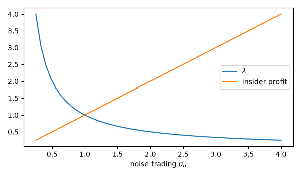
so the market’s depth \(1/\lambda\) rises with noise trading, the insider earns \(\sigma_v\sigma_u/2\) at the noise traders’ expense, and the price reveals exactly half of the insider’s information.

import matplotlib.pyplot as plt
import numpy as np

from financialkit.market_microstructure import kyle_equilibrium, kyle_lambda, simulate_kyle

eq = kyle_equilibrium(sigma_v=2.0, sigma_u=1.0, p0=50.0)
print(f"lambda {eq.lam}, beta {eq.beta}, insider profit {eq.insider_profit}, Var(v | p) {eq.posterior_variance}")

lambda 1.0, beta 0.5, insider profit 1.0, Var(v | p) 2.0

Order flow moves the price

Regressing the value on order flow across many auctions recovers the market maker’s lambda: the price is the best linear forecast of the value.

v, y, p = simulate_kyle(eq, 3000, rng=7)
fit = kyle_lambda(v - eq.p0, y)
fig, ax = plt.subplots(figsize=(6, 4))
ax.plot(y, v, ".", ms=2, color="0.6", label="value $v$")
ax.plot(np.sort(y), eq.p0 + eq.lam * np.sort(y), "C3", label=f"price, $\\lambda$ = {eq.lam}")
ax.set_xlabel("total order flow $y$")
ax.set_ylabel("price / value")
ax.set_title(f"fitted slope {fit.coef[1]:.3f} ± {fit.std_errors[1]:.3f}")
ax.legend()
fig.tight_layout()

The insider’s best response

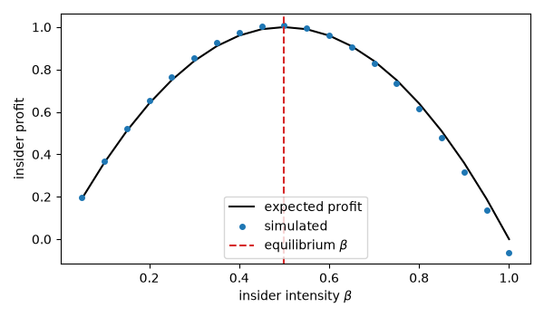
Given lambda, trading \(\beta(v - p_0)\) earns \(\beta\sigma_v^2(1 - \lambda\beta)\) on average, maximised at the equilibrium \(\beta = 1/(2\lambda)\): trading harder moves the price against itself.

betas = np.linspace(0.05, 1.0, 20)
sim_profit = [np.mean(b * (vv - eq.p0) * (vv - pp)) for b in betas for vv, _, pp in [simulate_kyle(eq, 4000, beta=b, rng=8)]]
fig, ax = plt.subplots(figsize=(6, 3.5))
ax.plot(betas, betas * eq.sigma_v**2 * (1 - eq.lam * betas), "k-", label="expected profit")
ax.plot(betas, sim_profit, "o", ms=4, color="C0", label="simulated")
ax.axvline(eq.beta, color="C3", ls="--", label="equilibrium $\\beta$")
ax.set_xlabel(r"insider intensity $\beta$")
ax.set_ylabel("insider profit")
ax.legend()
fig.tight_layout()

More noise, deeper market

sigma_u = np.linspace(0.25, 4, 50)
fig, ax = plt.subplots(figsize=(6, 3.5))
ax.plot(sigma_u, [kyle_equilibrium(2.0, s).lam for s in sigma_u], label=r"$\lambda$")
ax.plot(sigma_u, [kyle_equilibrium(2.0, s).insider_profit for s in sigma_u], label="insider profit")
ax.set_xlabel(r"noise trading $\sigma_u$")
ax.legend()
fig.tight_layout()

plt.show()