Hasbrouck’s trade-impact VAR

Joel Hasbrouck (1991) measured the information in trades with a vector autoregression of quote revisions \(r_t\) and signed trades \(x_t\). Order flow is persistent and quotes also react to inventory, so a trade’s immediate price effect overstates what it reveals. The cumulative impulse response of the quote to an unexpected trade separates the two: it settles at the permanent impact, the information content, after the transitory part has decayed.

import matplotlib.pyplot as plt
import numpy as np

from financialkit.market_microstructure import hasbrouck_var
from financialkit.market_microstructure.visualizers import plot_impulse_response

rng = np.random.default_rng(10)

A market with informative, persistent, and inventory-driven trades

Buy and sell runs persist (each trade repeats the last sign with probability 0.75). Only the surprise in each trade moves the efficient price, by 2 cents; the dealer also shades the quote by 1.5 cents per trade for inventory, and works it off at 30% per trade.

n, lam = 20000, 0.02
x = np.empty(n)
x[0] = 1.0
for t in range(1, n):
    x[t] = x[t - 1] if rng.random() < 0.75 else -x[t - 1]
surprise = x - 0.5 * np.concatenate([[0.0], x[:-1]])  # E[x_t | x_t-1] = 0.5 x_t-1
efficient = np.cumsum(lam * surprise + 0.01 * rng.standard_normal(n))
inventory_shade = np.zeros(n)
for t in range(1, n):
    inventory_shade[t] = 0.7 * inventory_shade[t - 1] + 0.015 * x[t]
quote = efficient + inventory_shade
r = np.diff(quote)
res = hasbrouck_var(r, x[1:], lags=10, horizon=25)
print(f"immediate impact {res.impulse[0]:.4f}, permanent impact {res.permanent_impact:.4f} (true {lam})")
print(f"share of efficient-price variance due to trades {res.trade_share:.2f}")
ax = plot_impulse_response(res)
ax.axhline(lam, color="k", lw=0.8, ls=":", label="true information content")
ax.legend(fontsize="small")

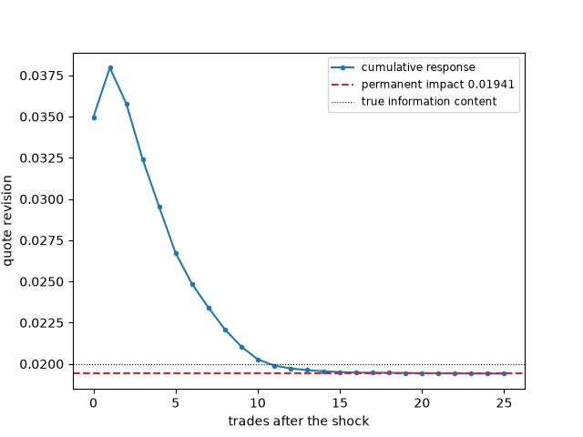
immediate impact 0.0350, permanent impact 0.0194 (true 0.02)
share of efficient-price variance due to trades 0.71

<matplotlib.legend.Legend object at 0x116e7eba0>

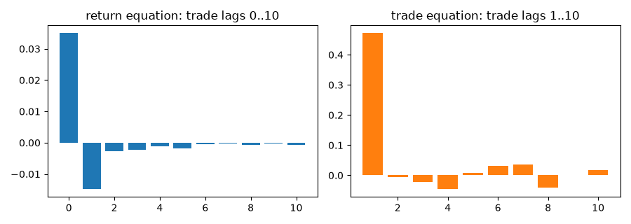
The VAR coefficients

fig, axes = plt.subplots(1, 2, figsize=(9, 3.2))
axes[0].bar(range(11), res.coef_r[[0, *range(11, 21)]], color="C0")
axes[0].set_title("return equation: trade lags 0..10")
axes[1].bar(range(1, 11), res.coef_x[10:], color="C1")
axes[1].set_title("trade equation: trade lags 1..10")
fig.tight_layout()

plt.show()