Easley, Kiefer, O’Hara and Paperman: the probability of informed trading

Easley, Kiefer, O’Hara and Paperman (1996) turned the Glosten-Milgrom logic into an estimator that needs only daily counts of buys and sells. On a day with private news (probability \(\alpha\)), informed traders add rate \(\mu\) to one side; otherwise only uninformed buys and sells arrive, at rates \(\varepsilon_b, \varepsilon_s\). The fitted mixture gives the share of trades that are informed, \(\mathrm{PIN} = \alpha\mu / (\alpha\mu + \varepsilon_b + \varepsilon_s)\). Their finding: thinly traded stocks have a higher PIN, which explains their wider spreads.

import matplotlib.pyplot as plt
import numpy as np

from financialkit.market_microstructure import fit_pin, simulate_pin

Three kinds of days

true = dict(alpha=0.35, delta=0.45, mu=60.0, eps_b=80.0, eps_s=75.0)
B, S = simulate_pin(250, **true, rng=11)
res = fit_pin(B, S)
pin_true = true["alpha"] * true["mu"] / (true["alpha"] * true["mu"] + true["eps_b"] + true["eps_s"])
print(f"alpha {res.alpha:.3f}, delta {res.delta:.3f}, mu {res.mu:.1f}, eps_b {res.eps_b:.1f}, eps_s {res.eps_s:.1f}")
print(f"PIN {res.pin:.3f} ± {res.pin_se:.3f} (true {pin_true:.3f})")

fig, ax = plt.subplots(figsize=(5, 5))
ax.plot(B, S, ".", color="0.4")
for (cb, cs), name in [((res.eps_b, res.eps_s), "no news"), ((res.eps_b, res.eps_s + res.mu), "bad news"), ((res.eps_b + res.mu, res.eps_s), "good news")]:
    ax.plot(cb, cs, "o", ms=12, mfc="none", mew=2, label=name)
ax.set_xlabel("buys per day")
ax.set_ylabel("sells per day")
ax.legend()
fig.tight_layout()

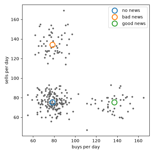
alpha 0.391, delta 0.572, mu 58.8, eps_b 78.4, eps_s 75.5
PIN 0.130 ± 0.009 (true 0.119)

Active and inactive stocks

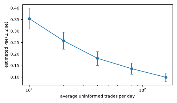
Uninformed volume scales up across stocks while information events stay similar, so PIN falls with activity, as in the paper’s volume deciles.

scales = [0.25, 0.5, 1.0, 2.0, 4.0]
pins = []
for i, sc in enumerate(scales):
    b_, s_ = simulate_pin(250, 0.3, 0.5, 30.0 * np.sqrt(sc), 20.0 * sc, 20.0 * sc, rng=20 + i)
    pins.append(fit_pin(b_, s_))
fig, ax = plt.subplots(figsize=(6, 3.5))
ax.errorbar([40 * s for s in scales], [p.pin for p in pins], yerr=[2 * p.pin_se for p in pins], fmt="o-", capsize=3)
ax.set_xscale("log")
ax.set_xlabel("average uninformed trades per day")
ax.set_ylabel("estimated PIN (± 2 se)")
fig.tight_layout()

plt.show()