Glosten and Milgrom: a spread from adverse selection alone

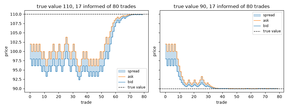
Lawrence Glosten and Paul Milgrom (1985) explained the spread with no inventory and no costs. A competitive dealer trades one unit at a time with traders who are informed with probability \(\alpha\). Since a buy is more likely to come from someone who knows the value is high, the dealer sets the ask to \(E[V \mid \text{buy}]\) and the bid to \(E[V \mid \text{sell}]\), losing to the informed exactly what it gains from the uninformed. Each trade updates the dealer’s belief by Bayes’ rule, so prices are a martingale that converges to the truth.

import matplotlib.pyplot as plt
import numpy as np

from financialkit.market_microstructure import glosten_milgrom_quotes, simulate_glosten_milgrom
from financialkit.market_microstructure.visualizers import plot_glosten_milgrom

Learning from the order flow

fig, axes = plt.subplots(1, 2, figsize=(10, 3.8), sharey=True)
for ax, value in zip(axes, (110.0, 90.0), strict=True):
    res = simulate_glosten_milgrom(80, alpha=0.2, v_low=90.0, v_high=110.0, true_value=value, rng=9)
    plot_glosten_milgrom(res, ax=ax)
    ax.set_title(f"true value {value:g}, {res.informed.sum()} informed of 80 trades")
fig.tight_layout()

More informed traders, wider spread

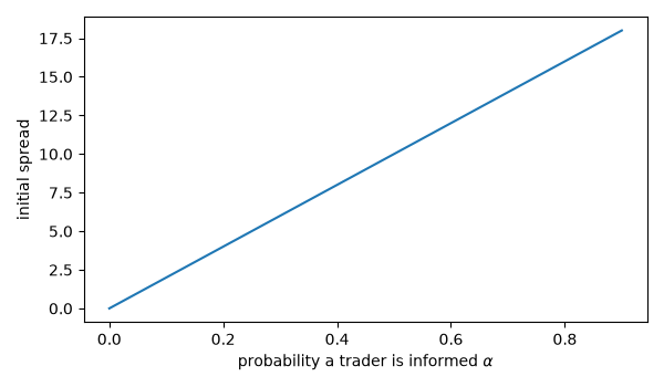
At the start (belief 1/2) the spread grows linearly with the share of informed traders; a dealer facing only informed traders would not trade.

alphas = np.linspace(0, 0.9, 46)
b, a = np.array([glosten_milgrom_quotes(0.5, al, 90.0, 110.0) for al in alphas]).T
fig, ax = plt.subplots(figsize=(6, 3.5))
ax.plot(alphas, a - b)
ax.set_xlabel(r"probability a trader is informed $\alpha$")
ax.set_ylabel("initial spread")
fig.tight_layout()

Faster learning with more informed trading

fig, ax = plt.subplots(figsize=(6, 3.5))
for al in (0.05, 0.2, 0.5):
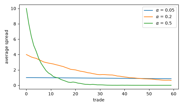
    runs = [simulate_glosten_milgrom(60, al, 90.0, 110.0, rng=seed) for seed in range(200)]
    spreads = np.mean([r.ask - r.bid for r in runs], axis=0)
    ax.plot(spreads, label=f"$\\alpha$ = {al}")
ax.set_xlabel("trade")
ax.set_ylabel("average spread")
ax.legend()
fig.tight_layout()

plt.show()