Cornish-Fisher: VaR beyond the normal

Cornish and Fisher (1937) expanded the quantile of a nearly normal distribution in its cumulants. To second order, with skewness \(S\) and excess kurtosis \(K\),

\[z_{cf} = z + \frac{(z^2 - 1) S}{6} + \frac{(z^3 - 3z) K}{24} - \frac{(2z^3 - 5z) S^2}{36},\]

so a VaR needs only four sample moments to account for crash-prone skew and fat tails. The expansion is accurate for moderate departures from normality and breaks down when the tails are very heavy.

import matplotlib.pyplot as plt
import numpy as np
from scipy import stats

from financialkit.risk import cornish_fisher_var, historical_var, parametric_var

A negatively skewed, fat-tailed return

Minus a gamma variable: losses are rarer than gains but larger. We compare the exact 99% VaR with the normal and Cornish-Fisher figures as the shape parameter, and so the skew, varies.

shapes = np.array([2.0, 4.0, 8.0, 16.0, 64.0])
alpha = 0.99
rows = []
for a in shapes:
    d = stats.gamma(a)
    mu, var, skew, kurt = (float(m) for m in d.stats(moments="mvsk"))
    exact = d.ppf(alpha) - mu  # loss quantile of mu - G
    rows.append((-skew, kurt, exact, parametric_var(0.0, np.sqrt(var), alpha), cornish_fisher_var(0.0, np.sqrt(var), -skew, kurt, alpha)))
print(" skew   kurt   exact  normal      CF")
for r in rows:
    print(" ".join(f"{v:6.3f}" for v in r))

 skew   kurt   exact  normal      CF
-1.414  3.000  4.638  3.290  4.688
-1.000  1.500  6.045  4.653  6.072
-0.707  0.750  8.000  6.580  8.014
-0.500  0.375 10.743  9.305 10.750
-0.250  0.094 20.067 18.611 20.069

From sample moments

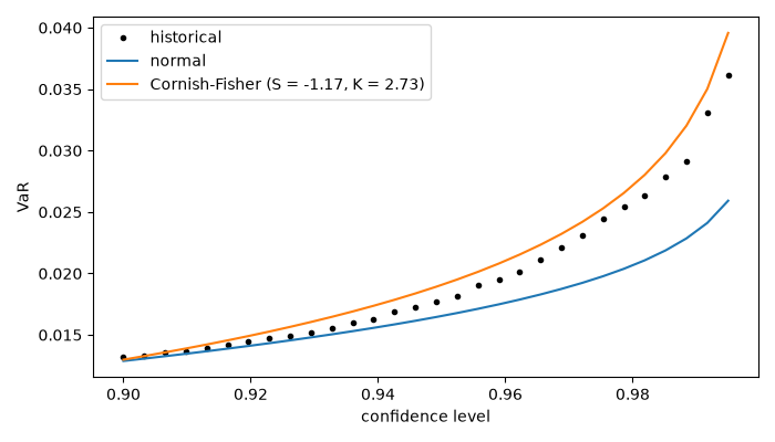
In practice the moments come from data. On 2,000 skewed returns the Cornish-Fisher VaR tracks the empirical quantile across confidence levels, where the normal VaR understates every one.

rng = np.random.default_rng(1)
x = 0.01 * (4.0 - stats.gamma(4.0).rvs(2000, random_state=rng)) / 2.0
m, s = x.mean(), x.std()
S, K = stats.skew(x), stats.kurtosis(x)
levels = np.linspace(0.9, 0.995, 30)
fig, ax = plt.subplots(figsize=(7, 4))
ax.plot(levels, [historical_var(x, a).var for a in levels], "k.", label="historical")
ax.plot(levels, parametric_var(m, s, levels), label="normal")
ax.plot(levels, cornish_fisher_var(m, s, S, K, levels), label=f"Cornish-Fisher (S = {S:.2f}, K = {K:.2f})")
ax.set_xlabel("confidence level")
ax.set_ylabel("VaR")
ax.legend()
fig.tight_layout()

plt.show()