RiskMetrics: parametric (delta-normal) VaR

In October 1994 J.P. Morgan published RiskMetrics, its methodology and daily covariance data, free. A portfolio with money exposures \(w\) to factors with covariance \(\Sigma\) has, under joint normality,

\[\mathrm{VaR}_\alpha = z_\alpha \sqrt{h\, w^\top \Sigma w},\]

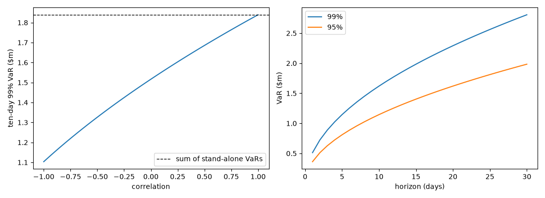
computable in a spreadsheet for a whole bank. Diversification is explicit: the portfolio VaR is less than the sum of the stand-alone VaRs unless every correlation is one.

import matplotlib.pyplot as plt
import numpy as np

from financialkit.risk import delta_normal_var, parametric_var

Hull’s two-asset example

Hull (Options, Futures, and Other Derivatives, 10th ed., Ch. 22): $10 million of Microsoft (2% daily volatility) and $5 million of AT&T (1%), correlation 0.3.

w = np.array([10e6, 5e6])
vols = np.array([0.02, 0.01])
cov = np.array([[1.0, 0.3], [0.3, 1.0]]) * np.outer(vols, vols)
stand_alone = [parametric_var(0.0, wi * si, 0.99, horizon=10) for wi, si in zip(w, vols, strict=True)]
total = delta_normal_var(w, cov, 0.99, horizon=10)
print(f"ten-day 99% VaR: Microsoft {stand_alone[0]:,.0f}, AT&T {stand_alone[1]:,.0f}")
print(f"portfolio {total:,.0f}; diversification benefit {sum(stand_alone) - total:,.0f}")

ten-day 99% VaR: Microsoft 1,471,312, AT&T 367,828
portfolio 1,620,114; diversification benefit 219,026

Diversification and the square-root-of-time rule

rho = np.linspace(-1, 1, 81)
var_rho = [delta_normal_var(w, np.array([[1.0, c], [c, 1.0]]) * np.outer(vols, vols), 0.99, 10) for c in rho]
h = np.arange(1, 31)
fig, axes = plt.subplots(1, 2, figsize=(11, 4))
axes[0].plot(rho, np.array(var_rho) / 1e6)
axes[0].axhline(sum(stand_alone) / 1e6, color="k", ls="--", lw=1, label="sum of stand-alone VaRs")
axes[0].set_xlabel("correlation")
axes[0].set_ylabel("ten-day 99% VaR ($m)")
axes[0].legend()
axes[1].plot(h, [delta_normal_var(w, cov, 0.99, k) / 1e6 for k in h], label="99%")
axes[1].plot(h, [delta_normal_var(w, cov, 0.95, k) / 1e6 for k in h], label="95%")
axes[1].set_xlabel("horizon (days)")
axes[1].set_ylabel("VaR ($m)")
axes[1].legend()
fig.tight_layout()

plt.show()