Boudoukh-Richardson-Whitelaw hybrid VaR

Historical simulation gives every day in the window the same weight, so after a jump in volatility it takes months to notice and then drops the crisis days abruptly when they leave the window. Boudoukh, Richardson and Whitelaw (1998) weighted the outcome \(i\) days old by \(\lambda^i\), combining RiskMetrics’ exponential smoothing with historical simulation’s distribution-free tail: “the best of both worlds”.

import matplotlib.pyplot as plt
import numpy as np

from financialkit.risk import historical_var, hybrid_var
from financialkit.risk.visualizers import plot_var

rng = np.random.default_rng(11)
vol = np.r_[np.full(500, 0.008), np.full(150, 0.025), np.full(350, 0.008)]
pnl = vol * rng.standard_t(5, vol.size) / np.sqrt(5 / 3)
window = 250

Rolling forecasts through a turbulent spell

days = np.arange(window, pnl.size)
hs = [historical_var(pnl[t - window : t], 0.99).var for t in days]
bw = [hybrid_var(pnl[t - window : t], 0.99, lam=0.98).var for t in days]
fig, ax = plt.subplots(figsize=(8, 3.8))
ax.plot(np.arange(pnl.size), pnl, color="0.75", lw=0.6)
ax.plot(days, -np.array(hs), label="historical (equal weights)")
ax.plot(days, -np.array(bw), label="hybrid, lambda = 0.98")
ax.plot(np.arange(pnl.size), -2.326 * vol, "k:", lw=1, label="true 99% normal-equivalent")
ax.set_xlabel("day")
ax.set_ylabel("P&L and minus VaR")
ax.legend(loc="lower left", fontsize=8)
fig.tight_layout()

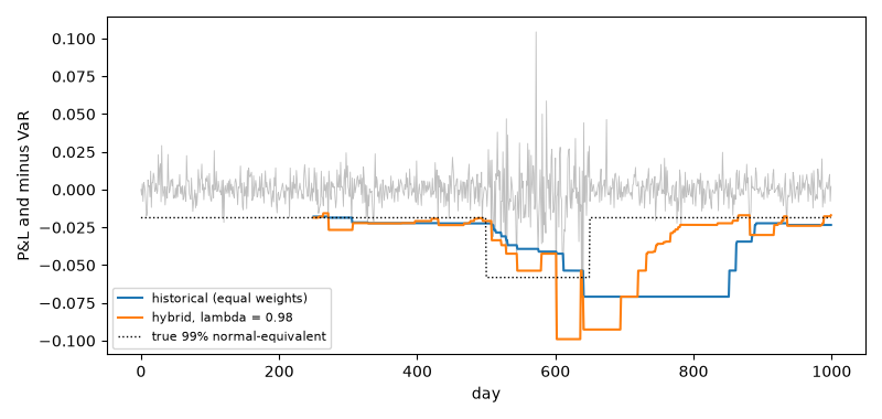
The weighted distribution on the first turbulent days

Twenty days into the turbulent period the hybrid method already puts a third of its probability mass on them.

t = 520
res = hybrid_var(pnl[t - window : t], 0.99, 0.98)
print(f"weight on last 20 days: {res.weights[-20:].sum():.2f}  (equal weighting: {20 / window:.2f})")
plot_var(res)

plt.show()

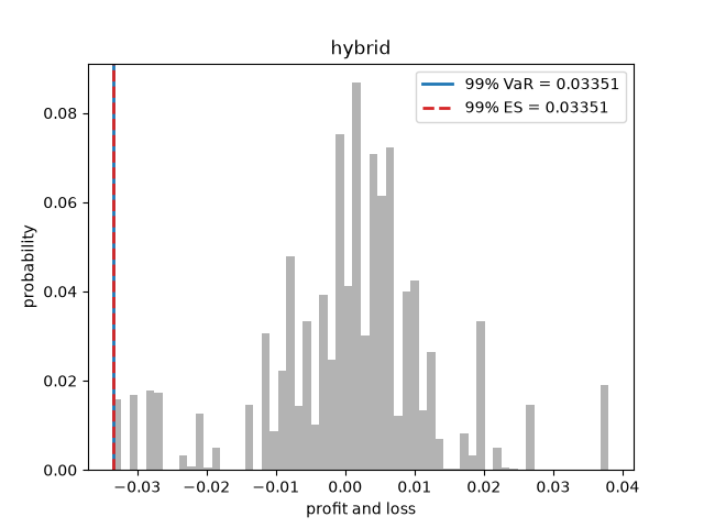
weight on last 20 days: 0.33  (equal weighting: 0.08)