Roy’s safety-first criterion

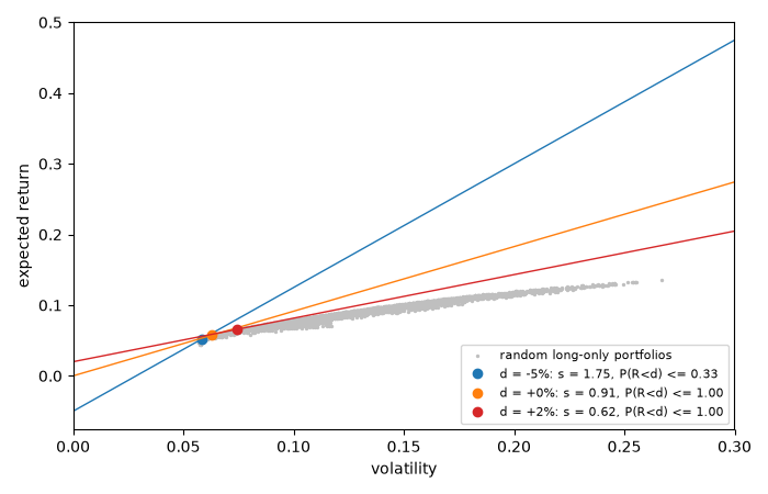
The same year as Markowitz, A. D. Roy (1952) asked which portfolio minimises the chance of disaster, \(P(R < d)\). With only means and variances known, Chebyshev’s inequality bounds it by \(1 / s^2\), where \(s = (\mu - d)/\sigma\), so the safest portfolio maximises \(s\): the point where a line from \((0, d)\) touches the efficient frontier. It is the first downside risk measure and an early form of the Sharpe ratio.

import matplotlib.pyplot as plt
import numpy as np

from financialkit.risk import safety_first_portfolio, safety_first_ratio, shortfall_probability

mu = np.array([0.04, 0.07, 0.10, 0.14])
vol = np.array([0.06, 0.12, 0.18, 0.28])
corr = np.array([[1.0, 0.2, 0.1, 0.0], [0.2, 1.0, 0.4, 0.3], [0.1, 0.4, 1.0, 0.5], [0.0, 0.3, 0.5, 1.0]])
cov = corr * np.outer(vol, vol)

The frontier and Roy’s tangent

rng = np.random.default_rng(0)
W = rng.dirichlet(np.ones(4), 4000)
port_mu, port_sd = W @ mu, np.sqrt(np.einsum("ij,jk,ik->i", W, cov, W))
fig, ax = plt.subplots(figsize=(7, 4.5))
ax.scatter(port_sd, port_mu, s=2, c="0.75", label="random long-only portfolios")
for d, color in [(-0.05, "C0"), (0.0, "C1"), (0.02, "C3")]:
    w = safety_first_portfolio(mu, cov, d)
    m, s = w @ mu, np.sqrt(w @ cov @ w)
    sr = safety_first_ratio(m, s, d)
    xs = np.linspace(0, 0.3, 2)
    ax.plot(xs, d + sr * xs, color=color, lw=1)
    ax.plot(s, m, "o", color=color, label=f"d = {d:+.0%}: s = {sr:.2f}, P(R<d) <= {shortfall_probability(m, s, d):.2f}")
ax.set_xlabel("volatility")
ax.set_ylabel("expected return")
ax.set_xlim(0, 0.3)
ax.legend(fontsize=8, loc="lower right")
fig.tight_layout()

Chebyshev’s bound against the normal probability

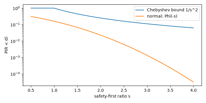
Roy’s bound holds for any distribution, which is why it is loose: for normal returns the true shortfall probability is far smaller.

s = np.linspace(0.5, 4, 100)
fig, ax = plt.subplots(figsize=(7, 3.5))
ax.semilogy(s, shortfall_probability(s, 1.0, 0.0), label="Chebyshev bound 1/s^2")
ax.semilogy(s, shortfall_probability(s, 1.0, 0.0, "normal"), label="normal: Phi(-s)")
ax.set_xlabel("safety-first ratio s")
ax.set_ylabel("P(R < d)")
ax.legend()
fig.tight_layout()

plt.show()