Pritsker: Monte Carlo VaR for option books

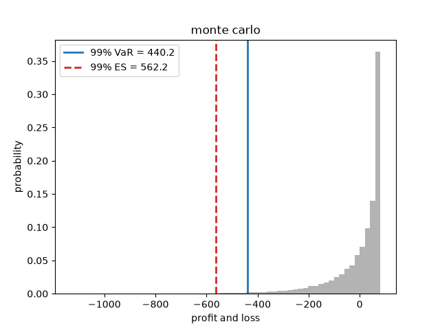
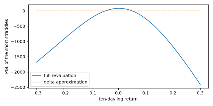
Delta-normal VaR treats every position as linear in its risk factors. For options that is badly wrong: a short straddle has zero delta at the money, so its delta-normal VaR is zero, yet it loses heavily on a large move in either direction. Pritsker (1997) compared delta, delta-gamma and full-revaluation Monte Carlo VaR and found that only full revaluation is reliable for books with large gamma. The cost is repricing every position in every scenario.

import matplotlib.pyplot as plt
import numpy as np

from financialkit.options import black_scholes_greeks, black_scholes_price
from financialkit.risk import delta_normal_var, monte_carlo_var
from financialkit.risk.visualizers import plot_var

S0, T, r, sigma = 100.0, 0.25, 0.03, 0.25
K = S0 * np.exp((r + 0.5 * sigma**2) * T)  # d1 = 0: the straddle is delta-neutral
h = 10 / 252
straddle = lambda S, t: black_scholes_price(S, K, t, r, sigma) + black_scholes_price(S, K, t, r, sigma, option_type="put")
value0 = straddle(S0, T)

Full revaluation against the delta approximation

The risk factor is the log return of the stock over ten days. The book is short 100 delta-neutral straddles.

def pnl(dX):
    return -100.0 * (straddle(S0 * np.exp(dX[:, 0]), T - h) - value0)


cov = np.array([[sigma**2]])
res = monte_carlo_var(pnl, cov, 0.99, horizon=h, n_paths=20_000, rng=0)
g = black_scholes_greeks(S0, K, T, r, sigma)
gp = black_scholes_greeks(S0, K, T, r, sigma, option_type="put")
delta = -100.0 * (g.delta + gp.delta) * S0
print(f"position delta (in $ per unit log return): {delta:,.1f}")
print(f"delta-normal 99% ten-day VaR: {delta_normal_var([delta], cov, 0.99, h):,.1f}")
print(f"Monte Carlo VaR {res.var:,.1f}  (95% CI {res.ci[0]:,.1f} to {res.ci[1]:,.1f}),  ES {res.es:,.1f}")
plot_var(res)

position delta (in $ per unit log return): -0.0
delta-normal 99% ten-day VaR: 0.0
Monte Carlo VaR 440.2  (95% CI 423.5 to 461.3),  ES 562.2

<Axes: title={'center': 'monte carlo'}, xlabel='profit and loss', ylabel='probability'>

The P&L profile behind it

x = np.linspace(-0.3, 0.3, 200)
fig, ax = plt.subplots(figsize=(7, 3.5))
ax.plot(x, pnl(x[:, None]), label="full revaluation")
ax.plot(x, delta * x, "--", label="delta approximation")
ax.set_xlabel("ten-day log return")
ax.set_ylabel("P&L of the short straddles")
ax.legend()
fig.tight_layout()

plt.show()