Merton’s jump diffusion

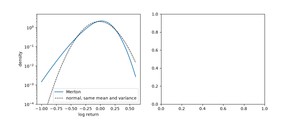
Robert Merton (1976) added Poisson jumps with lognormal sizes to geometric Brownian motion. If the jump risk is diversifiable it is not priced, and conditioning on the number of jumps turns the option into a Poisson mixture of Black-Scholes prices with adjusted rates and volatilities. Jumps fatten the tails of the return distribution, and because a few jumps matter far more over a week than over five years, they make short-dated smiles much steeper than long-dated ones.

import matplotlib.pyplot as plt
import numpy as np
from scipy.stats import norm

from financialkit.stochastic_volatility import MertonJumpModel, cos_density, merton_jump_price
from financialkit.stochastic_volatility.visualizers import plot_density, plot_smile

S, r = 100.0, 0.03
m = MertonJumpModel(sigma=0.15, lam=0.5, mu_j=-0.15, delta=0.1)

The series against simulation

x = m.sample_terminal(1.0, 200_000, rng=0)
pay = np.exp(-r) * np.maximum(S * np.exp(r) * np.exp(x) - 100.0, 0.0)
print(f"Merton series {merton_jump_price(S, 100.0, 1.0, r, m):.4f}, Monte Carlo {pay.mean():.4f} +/- {2 * pay.std() / np.sqrt(pay.size):.4f}")

Merton series 9.0558, Monte Carlo 9.0985 +/- 0.0555

Fat tails

grid = np.linspace(-1.0, 0.6, 400)
dens = cos_density(m, grid, 1.0)
c1, c2, _ = m.cumulants(1.0)
fig, (ax1, ax2) = plt.subplots(1, 2, figsize=(10, 4))
plot_density(grid, dens, ax=ax1, label="Merton", log=True)
ax1.plot(grid, norm.pdf(grid, c1, np.sqrt(c2)), "k--", lw=1, label="normal, same mean and variance")
ax1.set_ylim(1e-4, 5)
ax1.legend()

<matplotlib.legend.Legend object at 0x115114d70>

Smiles flatten with maturity

for T in (0.1, 0.5, 2.0):
    F = S * np.exp(r * T)
    K = F * np.exp(np.linspace(-0.35, 0.25, 25) * np.sqrt(T))
    plot_smile(K, m.implied_vol(S, K, T, r), forward=F, ax=ax2, label=f"T = {T}")
fig.tight_layout()

plt.show()