Madan, Carr and Chang’s skewed variance gamma

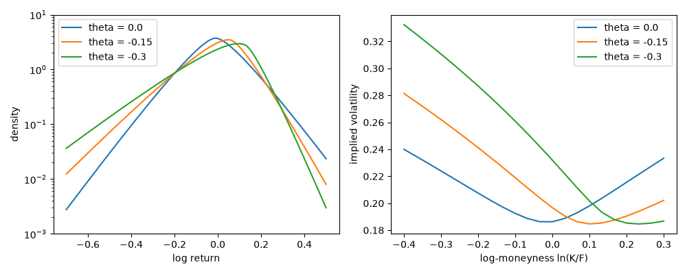
Madan, Carr and Chang (1998) added a drift \(\theta\) in business time: \(X = \theta G_t + \sigma W_{G_t}\). A negative \(\theta\) moves mass into the left tail, turning the symmetric Madan-Seneta smile into the equity skew with one extra parameter, and they priced options in closed form. Fang and Oosterlee (2008) later used one of their parameter sets as a benchmark; it is reproduced below.

import matplotlib.pyplot as plt
import numpy as np

from financialkit.stochastic_volatility import VarianceGammaModel, lewis_price
from financialkit.stochastic_volatility.visualizers import plot_density, plot_smile

m = VarianceGammaModel(sigma=0.12, nu=0.2, theta=-0.14)
for T, ref in ((0.1, 10.993703187), (1.0, 19.099354724)):
    print(f"T = {T}: call {lewis_price(m, 100.0, 90.0, T, 0.1):.9f} (Fang-Oosterlee reference {ref})")

T = 0.1: call 10.993703187 (Fang-Oosterlee reference 10.993703187)
T = 1.0: call 19.099354724 (Fang-Oosterlee reference 19.099354724)

The skew comes from theta

S, r, T = 100.0, 0.0, 0.5
x = np.linspace(-0.7, 0.5, 400)
K = S * np.exp(np.linspace(-0.4, 0.3, 22))
fig, (ax1, ax2) = plt.subplots(1, 2, figsize=(10, 4))
for theta in (0.0, -0.15, -0.3):
    v = VarianceGammaModel(0.2, 0.3, theta)
    plot_density(x, v.pdf(x, T), ax=ax1, label=f"theta = {theta}", log=True)
    plot_smile(K, v.implied_vol(S, K, T, r), forward=S, ax=ax2, label=f"theta = {theta}")
ax1.set_ylim(1e-3, 10)
fig.tight_layout()

plt.show()