Madan and Seneta’s variance gamma

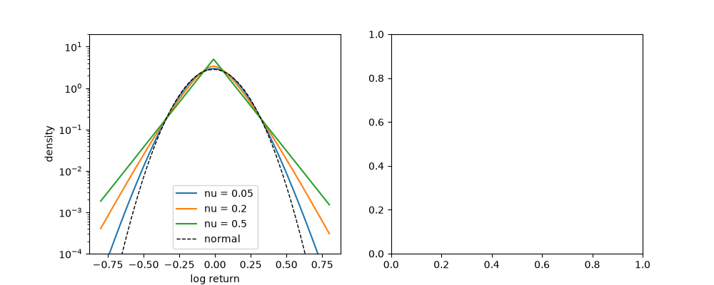
Madan and Seneta (1990) ran a Brownian motion on a random business clock: gamma-distributed time \(G_t\), with variance rate \(\nu\). The result, \(\sigma W_{G_t}\), is a pure-jump Lévy process with infinitely many small jumps, symmetric, and with tails heavier than the normal’s but lighter than a power law. The density is closed form in terms of a modified Bessel function. The clock’s variance \(\nu\) sets the excess kurtosis (\(3\nu/T\)).

import matplotlib.pyplot as plt
import numpy as np
from scipy.stats import norm

from financialkit.stochastic_volatility import VarianceGammaModel
from financialkit.stochastic_volatility.visualizers import plot_density, plot_smile

T, sigma = 0.5, 0.2
x = np.linspace(-0.8, 0.8, 401)

fig, (ax1, ax2) = plt.subplots(1, 2, figsize=(10, 4))
for nu in (0.05, 0.2, 0.5):
    m = VarianceGammaModel(sigma=sigma, nu=nu, theta=0.0)
    plot_density(x, m.pdf(x, T), ax=ax1, label=f"nu = {nu}", log=True)
ax1.plot(x, norm.pdf(x, -0.5 * sigma**2 * T, sigma * np.sqrt(T)), "k--", lw=1, label="normal")
ax1.set_ylim(1e-4, 20)
ax1.legend()

<matplotlib.legend.Legend object at 0x115224ad0>

Subordination: sampling and the density agree

m = VarianceGammaModel(sigma=sigma, nu=0.2, theta=0.0)
draws = m.sample_terminal(T, 100_000, rng=0)
print(f"sample excess kurtosis {np.mean((draws - draws.mean()) ** 4) / draws.var() ** 2 - 3:.2f}, theory 3 nu / T = {3 * 0.2 / T:.2f}")

sample excess kurtosis 1.19, theory 3 nu / T = 1.20

A symmetric smile

S, r = 100.0, 0.0
K = S * np.exp(np.linspace(-0.4, 0.4, 21))
for nu in (0.05, 0.2, 0.5):
    plot_smile(K, VarianceGammaModel(sigma, nu).implied_vol(S, K, T, r), forward=S, ax=ax2, label=f"nu = {nu}")
fig.tight_layout()

plt.show()