Bashforth and Adams: linear multistep methods

John Couch Adams, computing drop shapes for Francis Bashforth’s 1883 study of capillarity, reused the slopes already computed at earlier steps instead of throwing them away. Integrating the polynomial through the last \(k\) slopes gives the order-\(k\) Adams-Bashforth formula,

\[y_{n+1} = y_n + h \sum_{j=0}^{k-1} \beta_j f_{n-j}, \qquad \text{e.g. AB2: } y_{n+1} = y_n + h\bigl(\tfrac32 f_n - \tfrac12 f_{n-1}\bigr),\]

at the cost of one new evaluation of \(f\) per step, however high the order. The price appears in the method’s stability region, which shrinks as the order grows.

import matplotlib.pyplot as plt
import numpy as np

from mathematicskit.integrators import adams_bashforth_boundary_locus, adams_bashforth_integrate, njit, rk4_integrate
from mathematicskit.ode_dynamics.visualizers import plot_stability_regions


@njit
def oscillator(state, t, params):
    out = np.empty(2)
    out[0] = state[1]
    out[1] = -state[0]
    return out

Order k from one evaluation per step

Error at \(t = 2\pi\) for \(x'' = -x\), against the number of right-hand-side evaluations. RK4 needs four per step, so AB4 matches its order at a quarter of the cost per step.

fig, (ax0, ax1) = plt.subplots(1, 2, figsize=(12, 4.8))
steps = np.array([50, 100, 200, 400, 800, 1600])
y0, t_end = np.array([1.0, 0.0]), 2.0 * np.pi
for order in (1, 2, 3, 4):
    errors = [np.abs(adams_bashforth_integrate(oscillator, y0, 0.0, t_end / n, n, np.zeros(1), order)[1][-1] - y0).max() for n in steps]
    ax0.loglog(steps, errors, "o-", label=f"AB{order}")
    print(f"AB{order}: error ratio for halved h = {errors[-2] / errors[-1]:.2f} (2^{order} = {2**order})")
rk4_errors = [np.abs(rk4_integrate(oscillator, y0, 0.0, t_end / n, n, np.zeros(1))[1][-1] - y0).max() for n in steps]
ax0.loglog(4 * steps, rk4_errors, "k^--", label="RK4")
ax0.set_xlabel("right-hand-side evaluations")
ax0.set_ylabel(r"max error at $t = 2\pi$")
ax0.set_title("Adams-Bashforth: order k at one evaluation per step")
ax0.legend()

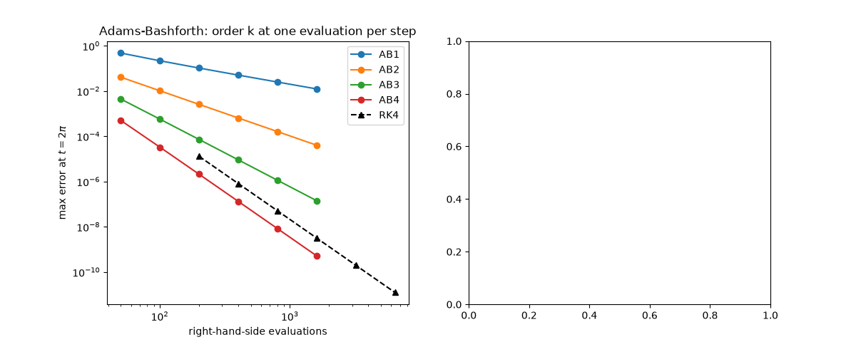
AB1: error ratio for halved h = 2.01 (2^1 = 2)
AB2: error ratio for halved h = 4.00 (2^2 = 4)
AB3: error ratio for halved h = 7.99 (2^3 = 8)
AB4: error ratio for halved h = 15.97 (2^4 = 16)

<matplotlib.legend.Legend object at 0x7fd7c5ab66f0>

Stability regions shrink with order

Shaded: the absolute-stability regions in the \(z = \lambda h\) plane. Dashed: the boundary locus \(z(\theta) = \rho(e^{i\theta})/\sigma(e^{i\theta})\), the curve on which a root of the characteristic polynomial lies on the unit circle. The real stability interval is \([-2, 0]\) for AB1 (Euler), \([-1, 0]\) for AB2, \([-6/11, 0]\) for AB3, and \([-3/10, 0]\) for AB4.

plot_stability_regions(
    ["euler", "adams_bashforth2", "adams_bashforth3", "adams_bashforth4"],
    ax=ax1,
    re_range=(-2.3, 0.6),
    im_range=(-1.4, 1.4),
    labels=["AB1 (Euler)", "AB2", "AB3", "AB4"],
)
for order in (1, 2, 3, 4):
    locus = adams_bashforth_boundary_locus(order)
    ax1.plot(locus.real, locus.imag, "--", color=f"C{order - 1}", lw=0.8)
ax1.set_xlim(-2.3, 0.6)
ax1.set_ylim(-1.4, 1.4)
fig.tight_layout()

plt.show()