Examples#
This gallery walks through every public feature of mathematicskit.numerical_analysis:
scalar root finding with convergence-order verification and
acceleration, polynomial interpolation (Lagrange, Newton
divided-difference, Hermite, cubic splines, Chebyshev nodes), function
approximation (Bernstein, Padé, Remez minimax), polynomial evaluation and
root conditioning, compensated summation, and least-squares polynomial
regression.
See also the narrative tutorial:
Each script in this gallery is self-contained and can be run directly with
python examples/numerical_analysis/<section>/<script>.py. Every script also
carries an RST module docstring as its title/description and uses # %%
markers to split narrative text from code, which is exactly what
Sphinx-Gallery renders into the pages below – the script is the source of
truth for what you see, not a copy of it.
Sections#
root_finding – bisection, Newton-Raphson, secant, and fixed-point iteration side by side on the same problem, with each method’s empirical convergence order verified against its theoretical rate; Halley’s cubic method; Aitken’s delta-squared process and Steffensen’s method; Newton’s method for nonlinear systems and Broyden’s quasi-Newton method.
interpolation – Lagrange and Newton divided-difference polynomial interpolation, shown to agree exactly and to reproduce any polynomial up to the interpolation degree; Hermite interpolation of values and slopes.
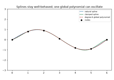
splines – natural and clamped cubic spline interpolation, and why a spline avoids the oscillation a single high-degree polynomial would show.
chebyshev – Chebyshev interpolation nodes and the Runge phenomenon: why equally spaced nodes can diverge as degree grows, and Chebyshev nodes don’t.
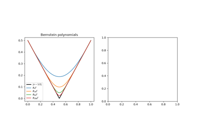
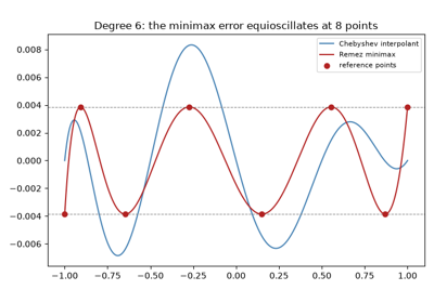
approximation – Bernstein polynomials and the Weierstrass theorem, Padé approximants, and Remez’s best uniform (minimax) approximation.
polynomials – Horner’s scheme with deflation, and Wilkinson’s ill-conditioned polynomial.
floating_point – IEEE 754 bit fields, machine epsilon and the spacing of floats, catastrophic cancellation in the quadratic formula, and Kahan’s compensated summation against naive and pairwise summation.
regression – least-squares polynomial regression via the normal equations, and how the fit’s condition number worsens with degree.
Function approximation#
Approximating a function over a whole interval: Bernstein polynomials and the Weierstrass theorem, Padé rational approximants, and Remez’s best uniform (minimax) polynomials.
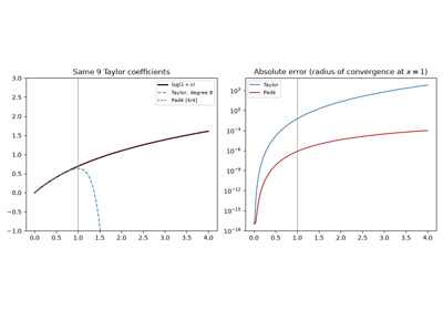
Padé approximants beyond the radius of convergence
Runge’s phenomenon and Chebyshev nodes#
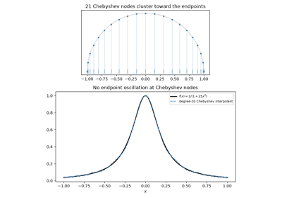
Why node placement matters: equally spaced interpolation nodes can make the error diverge as the polynomial degree grows (Runge’s 1901 example), while Chebyshev nodes keep the error shrinking.
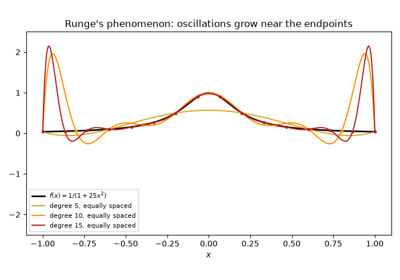
Runge’s phenomenon: equally spaced interpolation diverges
Floating-point arithmetic#
How IEEE 754 stores numbers, machine epsilon and the spacing of floats, catastrophic cancellation, and algorithms that compensate for rounding error.
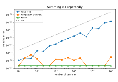
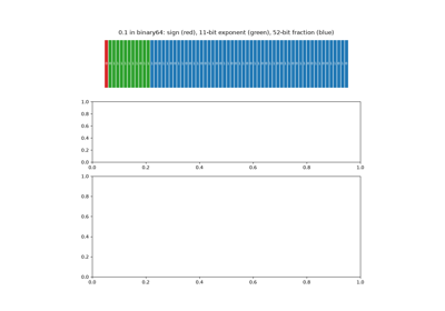
IEEE 754: bit layouts, machine epsilon, and the spacing of floats
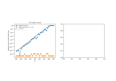
Forsythe’s quadratic formula: catastrophic cancellation
Interpolation#
Lagrange and Newton divided-difference polynomial interpolation: the same unique interpolating polynomial, built and evaluated two different ways.
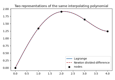
Lagrange vs. Newton divided-difference interpolation
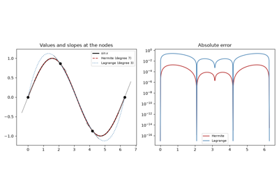
Hermite interpolation: matching slopes as well as values
Polynomials#
Evaluating polynomials efficiently with Horner’s scheme, and how sensitive their roots can be to tiny changes in the coefficients.
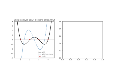
Horner’s method: evaluation, derivative, and deflation
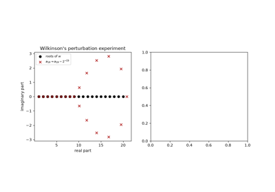
Least-squares regression#
Polynomial least-squares regression via the normal equations, and how the fit’s numerical conditioning worsens as the polynomial degree grows.
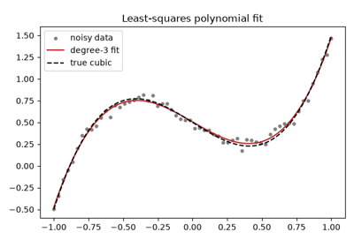
Least-squares polynomial regression and its conditioning
Root finding#
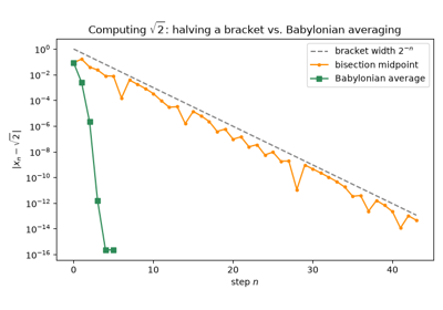
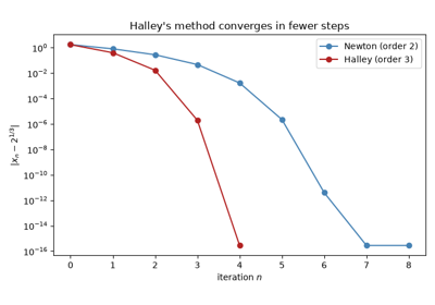
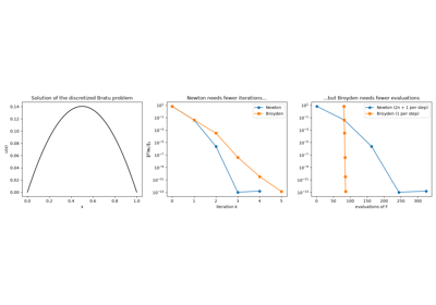
The Babylonian square-root rule and bisection, Newton-Raphson’s tangent iteration, Halley’s cubically convergent method, and Aitken/Steffensen acceleration, each with its empirical convergence order measured; then Newton’s method for systems of equations and Broyden’s quasi-Newton method, which saves the Jacobian evaluations.
An animation runs Newton against bisection on the graph of \(f\).
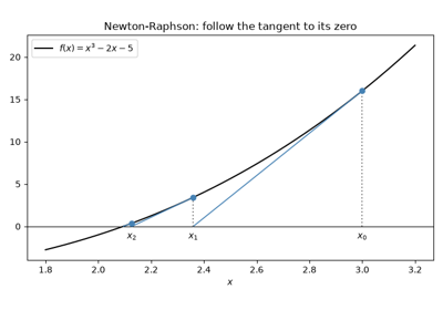
Newton-Raphson’s method: tangent lines and quadratic convergence
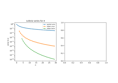
Aitken’s delta-squared process and Steffensen’s method
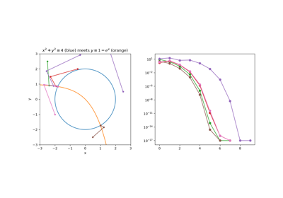
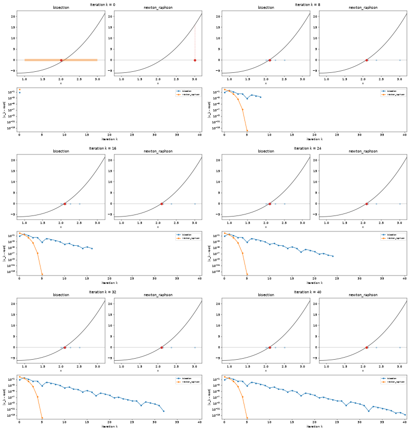
Animated: Newton’s tangents against bisection’s halving
Cubic splines#
Natural and clamped cubic spline interpolation, and how a piecewise cubic avoids the oscillation a single high-degree interpolating polynomial can show on the same data.