Chebyshev nodes: the cure for Runge’s phenomenon

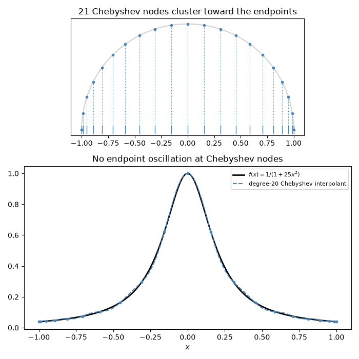
Chebyshev’s least-deviation polynomials suggest placing interpolation nodes at the extrema of \(T_n(x) = \cos(n \arccos x)\), which cluster toward the ends of \([-1, 1]\). At these nodes the Lebesgue constant grows only logarithmically, so the interpolant of Runge’s function \(1/(1+25x^2)\) converges as the degree rises. This script shows the node clustering, the degree-20 Chebyshev interpolant, and its error shrinking geometrically.

import matplotlib.pyplot as plt
import numpy as np

from mathematicskit.numerical_analysis import ChebyshevInterpolant, chebyshev_nodes, runge_function
from mathematicskit.numerical_analysis.systems.chebyshev import runge_phenomenon_errors
from mathematicskit.numerical_analysis.utils.error_analysis import lebesgue_constant

Nodes as projected equally spaced angles

The Chebyshev points are \(\cos(k\pi/(n-1))\): equally spaced points on the upper half circle, projected down onto \([-1, 1]\).

n = 21
nodes = chebyshev_nodes(n)
theta = np.linspace(0.0, np.pi, 200)

fig1, (ax_nodes, ax_fit) = plt.subplots(2, 1, figsize=(7, 7), gridspec_kw={"height_ratios": [1, 1.4]})
ax_nodes.plot(np.cos(theta), np.sin(theta), color="lightgray")
angles = np.arccos(np.clip(nodes, -1.0, 1.0))
for xk, tk in zip(nodes, angles):
    ax_nodes.plot([xk, xk], [0.0, np.sin(tk)], ":", color="steelblue", lw=0.8)
ax_nodes.plot(nodes, np.sin(angles), "o", ms=3, color="steelblue")
ax_nodes.plot(nodes, np.zeros_like(nodes), "|", ms=12, color="steelblue")
ax_nodes.set_aspect("equal")
ax_nodes.set_yticks([])
ax_nodes.set_title(f"{n} Chebyshev nodes cluster toward the endpoints")

x_fine = np.linspace(-1.0, 1.0, 600)
p_cheb = ChebyshevInterpolant(runge_function, n=n)
ax_fit.plot(x_fine, runge_function(x_fine), color="black", lw=2, label=r"$f(x) = 1/(1+25x^2)$")
ax_fit.plot(x_fine, p_cheb.evaluate(x_fine), "--", color="steelblue", label="degree-20 Chebyshev interpolant")
ax_fit.plot(nodes, runge_function(nodes), "o", ms=3, color="steelblue")
ax_fit.set_xlabel("$x$")
ax_fit.set_title("No endpoint oscillation at Chebyshev nodes")
ax_fit.legend(fontsize=8)
fig1.tight_layout()

Error now converges with degree

degrees = [5, 10, 20, 30, 40, 60]
_, chebyshev_errors = runge_phenomenon_errors(degrees)
for d, e in zip(degrees, chebyshev_errors):
    print(f"degree={d:2d}  Chebyshev max |error| = {e:.3e}")

fig2, ax2 = plt.subplots(figsize=(6, 4))
ax2.semilogy(degrees, chebyshev_errors, "o-", color="steelblue")
ax2.set_xlabel("polynomial degree")
ax2.set_ylabel(r"$\max |f - p_n|$")
ax2.set_title("Chebyshev-node interpolation error decays geometrically")
fig2.tight_layout()

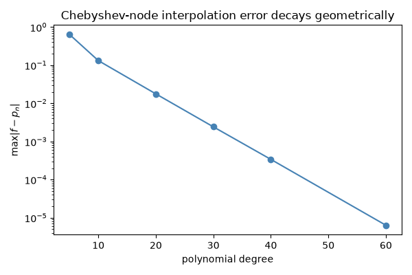
degree= 5  Chebyshev max |error| = 6.386e-01
degree=10  Chebyshev max |error| = 1.322e-01
degree=20  Chebyshev max |error| = 1.774e-02
degree=30  Chebyshev max |error| = 2.425e-03
degree=40  Chebyshev max |error| = 3.399e-04
degree=60  Chebyshev max |error| = 6.372e-06

Logarithmic growth of the Lebesgue constant

Compared with \(\tfrac{2}{\pi}\log n + 1\), the classical bound.

for nv in (5, 10, 20, 40, 80):
    lam = lebesgue_constant(chebyshev_nodes(nv))
    print(f"n={nv:2d}  Lebesgue(Chebyshev) = {lam:.3f}   (2/pi) log n + 1 = {2 / np.pi * np.log(nv) + 1:.3f}")

plt.show()

n= 5  Lebesgue(Chebyshev) = 1.799   (2/pi) log n + 1 = 2.025
n=10  Lebesgue(Chebyshev) = 2.362   (2/pi) log n + 1 = 2.466
n=20  Lebesgue(Chebyshev) = 2.837   (2/pi) log n + 1 = 2.907
n=40  Lebesgue(Chebyshev) = 3.294   (2/pi) log n + 1 = 3.348
n=80  Lebesgue(Chebyshev) = 3.743   (2/pi) log n + 1 = 3.790