Least-squares polynomial regression and its conditioning

PolynomialRegression fits a degree-d polynomial by solving the normal equations \(V^T V c = V^T y\). This script fits noisy cubic data, checks the \(R^2\) and residuals, and then shows the fit’s condition number (estimated via power iteration on the normal-equations matrix) growing sharply with degree – squaring the design matrix’s own condition number is exactly why the normal-equations approach is eventually replaced by a QR-based least-squares solve in mathematicskit.linalg.

import matplotlib.pyplot as plt
import numpy as np

from mathematicskit.numerical_analysis import PolynomialRegression

Fit noisy cubic data

rng = np.random.default_rng(0)
x = np.linspace(-1.0, 1.0, 60)
y_true = 2.0 * x**3 - x + 0.5
y = y_true + rng.normal(0.0, 0.05, x.shape)

model = PolynomialRegression(x, y, degree=3)
result = model.fit()
print(f"coefficients (highest power first): {result.coefficients}")
print(f"R^2 = {result.r_squared:.5f}, adjusted R^2 = {result.adjusted_r_squared:.5f}")

x_fine = np.linspace(-1.0, 1.0, 300)
fig1, ax1 = plt.subplots(figsize=(6, 4))
ax1.scatter(x, y, s=12, color="gray", label="noisy data")
ax1.plot(x_fine, model.predict(x_fine), color="firebrick", label="degree-3 fit")
ax1.plot(x_fine, 2.0 * x_fine**3 - x_fine + 0.5, "--", color="black", label="true cubic")
ax1.legend()
ax1.set_title("Least-squares polynomial fit")
fig1.tight_layout()

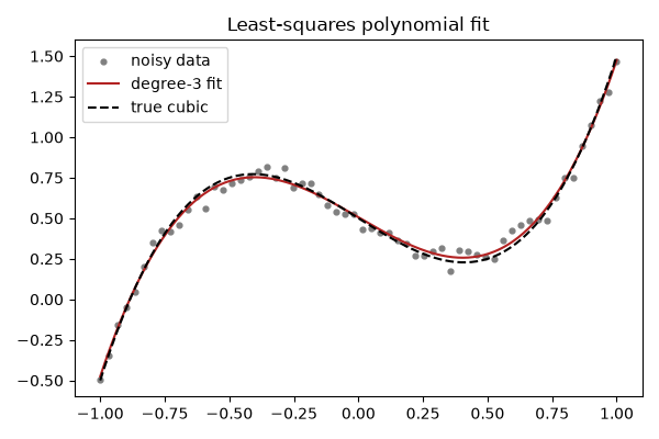
coefficients (highest power first): [ 1.90017422 -0.00562603 -0.92442784  0.50580371]
R^2 = 0.98524, adjusted R^2 = 0.98445

Conditioning worsens with degree

Fitting increasingly high-degree polynomials to the same data makes the Vandermonde normal-equations matrix more ill-conditioned.

degrees = [1, 2, 4, 6, 8, 10]
conditions = [PolynomialRegression(x, y, degree=d).fit().condition_number for d in degrees]
for d, c in zip(degrees, conditions):
    print(f"degree={d:2d}  condition number~{c:.3e}")

fig2, ax2 = plt.subplots(figsize=(6, 4))
ax2.semilogy(degrees, conditions, "o-", color="steelblue")
ax2.set_xlabel("polynomial degree")
ax2.set_ylabel("condition number of V^T V")
ax2.set_title("Normal-equations conditioning worsens with degree")
fig2.tight_layout()

plt.show()

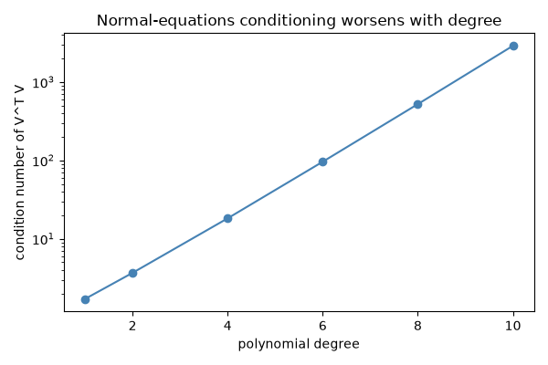
degree= 1  condition number~1.703e+00
degree= 2  condition number~3.666e+00
degree= 4  condition number~1.817e+01
degree= 6  condition number~9.583e+01
degree= 8  condition number~5.204e+02
degree=10  condition number~2.884e+03