Simpson’s Newton method for systems of equations

Thomas Simpson’s 1740 Essays stated Newton’s method in terms of fluxions and applied it to two equations in two unknowns. In matrix form, linearize \(F: \mathbb R^n \to \mathbb R^n\) at the current guess and solve for the step:

\[J(\mathbf x_k)\,\mathbf s_k = -F(\mathbf x_k), \qquad \mathbf x_{k+1} = \mathbf x_k + \mathbf s_k .\]

Here \(F(x, y) = (x^2 + y^2 - 4,\; e^x + y - 1)\): the circle of radius 2 meets the curve \(y = 1 - e^x\) twice. Each starting point is drawn to one intersection, and near it the residual is roughly squared at every step.

import matplotlib.pyplot as plt
import numpy as np

from mathematicskit.numerical_analysis import NewtonSystem


def F(v):
    x, y = v
    return np.array([x**2 + y**2 - 4.0, np.exp(x) + y - 1.0])


def J(v):
    x, y = v
    return np.array([[2.0 * x, 2.0 * y], [np.exp(x), 1.0]])

Iterate paths in the plane

starts = [(-2.5, 2.5), (-0.5, 2.0), (2.5, 0.5), (0.5, -2.5), (-2.0, -1.0)]
fig, (ax0, ax1) = plt.subplots(1, 2, figsize=(12, 5))
xs = np.linspace(-3, 3, 400)
X, Y = np.meshgrid(xs, xs)
ax0.contour(X, Y, X**2 + Y**2 - 4.0, levels=[0.0], colors="tab:blue")
ax0.contour(X, Y, np.exp(X) + Y - 1.0, levels=[0.0], colors="tab:orange")
for k, start in enumerate(starts):
    result = NewtonSystem(F, start, jacobian=J, tol=1e-14).solve()
    ax0.plot(result.history[:, 0], result.history[:, 1], "o-", ms=4, color=f"C{k + 2}")
    ax1.semilogy(result.residual_norms + 1e-17, "o-", color=f"C{k + 2}", label=f"start {start}")
    print(f"start {start}: root ({result.root[0]:+.12f}, {result.root[1]:+.12f}) in {result.iterations} iterations")
ax0.set_xlim(-3, 3)
ax0.set_ylim(-3, 3)
ax0.set_aspect("equal")
ax0.set_xlabel("x")
ax0.set_ylabel("y")
ax0.set_title(r"$x^2 + y^2 = 4$ (blue) meets $y = 1 - e^x$ (orange)")

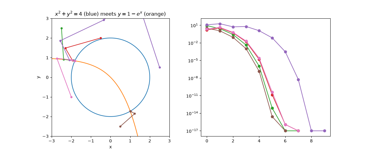
start (-2.5, 2.5): root (-1.816264068825, +0.837367799891) in 7 iterations
start (-0.5, 2.0): root (-1.816264068825, +0.837367799891) in 7 iterations
start (2.5, 0.5): root (-1.816264068825, +0.837367799891) in 9 iterations
start (0.5, -2.5): root (+1.004168738475, -1.729637287026) in 6 iterations
start (-2.0, -1.0): root (-1.816264068825, +0.837367799891) in 7 iterations

Text(0.5, 1.0, '$x^2 + y^2 = 4$ (blue) meets $y = 1 - e^x$ (orange)')

Quadratic convergence of the residual

ax1.set_xlabel("iteration k")
ax1.set_ylabel(r"$\|F(\mathbf{x}_k)\|_2$")
ax1.set_title("Correct digits roughly double per step")
ax1.legend(fontsize=8)
fig.tight_layout()

plt.show()