Natural and clamped cubic splines

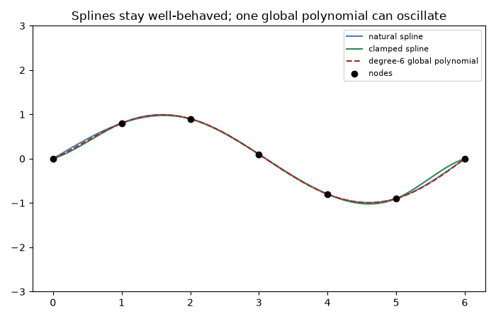
A cubic spline is a piecewise cubic through the data with continuous value, first, and second derivatives across nodes. A natural spline sets the curvature to zero at both ends; a clamped spline instead matches prescribed end-slopes. This script fits both to the same data and compares them against a single high-degree interpolating polynomial, which oscillates far more between nodes – the practical motivation for splines over one global polynomial.

import matplotlib.pyplot as plt
import numpy as np

from mathematicskit.numerical_analysis import CubicSpline, LagrangeInterpolant

Fit natural and clamped splines to the same data

x = np.array([0.0, 1.0, 2.0, 3.0, 4.0, 5.0, 6.0])
y = np.array([0.0, 0.8, 0.9, 0.1, -0.8, -0.9, 0.0])

natural = CubicSpline(x, y, boundary="natural")
clamped = CubicSpline(x, y, boundary="clamped", fpa=0.5, fpb=0.5)
global_poly = LagrangeInterpolant(x, y)

x_fine = np.linspace(x.min(), x.max(), 400)

fig, ax = plt.subplots(figsize=(7, 4.5))
ax.plot(x_fine, natural.evaluate(x_fine), color="steelblue", label="natural spline")
ax.plot(x_fine, clamped.evaluate(x_fine), color="seagreen", label="clamped spline")
ax.plot(x_fine, global_poly.evaluate(x_fine), "--", color="firebrick", label="degree-6 global polynomial")
ax.scatter(x, y, color="black", zorder=3, label="nodes")
ax.set_ylim(-3, 3)
ax.set_title("Splines stay well-behaved; one global polynomial can oscillate")
ax.legend(fontsize=8)
fig.tight_layout()

Natural boundary condition: zero curvature at both ends

second_derivs = natural.second_derivative_at_nodes()
print("S''(x_0), S''(x_n) for the natural spline:", second_derivs[0], second_derivs[-1])

plt.show()

S''(x_0), S''(x_n) for the natural spline: 0.0 8.881784197001252e-16