Newton-Raphson’s method: tangent lines and quadratic convergence

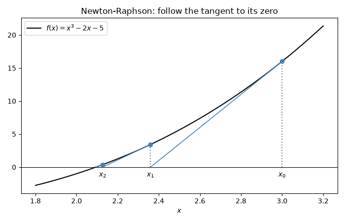
Newton and Raphson’s iteration replaces \(f\) by its tangent line at the current guess and steps to where that line crosses zero, \(x_{n+1} = x_n - f(x_n)/f'(x_n)\). This script draws the first tangent steps for \(f(x) = x^3 - 2x - 5\) (the cubic Newton himself used as his example) and shows the number of correct digits roughly doubling at every step, i.e. convergence of order 2.

import matplotlib.pyplot as plt
import numpy as np

from mathematicskit.numerical_analysis import NewtonRaphson, estimate_convergence_order

f = lambda x: x**3 - 2.0 * x - 5.0
fp = lambda x: 3.0 * x**2 - 2.0

result = NewtonRaphson(f, fp, x0=3.0, tol=1e-15).solve()
root = result.root
print(f"root = {root:.15f} after {result.iterations} iterations")

root = 2.094551481542327 after 7 iterations

Tangent-line steps

x = np.linspace(1.8, 3.2, 400)
fig1, ax1 = plt.subplots(figsize=(7, 4.5))
ax1.axhline(0.0, color="black", lw=0.8)
ax1.plot(x, f(x), color="black", label=r"$f(x) = x^3 - 2x - 5$")
for n, xn in enumerate(result.history[:3]):
    x_next = xn - f(xn) / fp(xn)
    ax1.plot([xn, x_next], [f(xn), 0.0], color="steelblue", lw=1.2)
    ax1.plot([xn, xn], [0.0, f(xn)], ":", color="gray")
    ax1.plot(xn, f(xn), "o", color="steelblue")
    ax1.annotate(f"$x_{n}$", (xn, 0.0), textcoords="offset points", xytext=(0, -14), ha="center")
ax1.set_xlabel("$x$")
ax1.set_title("Newton-Raphson: follow the tangent to its zero")
ax1.legend()
fig1.tight_layout()

Correct digits double every step

err = np.abs(result.history - root)
for n, e in enumerate(err):
    if e > 0:
        print(f"step {n}: error = {e:.2e}  correct digits ~ {-np.log10(e):.1f}")
print(f"empirical order ~ {estimate_convergence_order(result.history[:-1], root):.2f}")

fig2, ax2 = plt.subplots(figsize=(6, 4))
ax2.semilogy(np.where(err == 0, np.nan, err), "o-", color="steelblue")
ax2.set_xlabel("iteration $n$")
ax2.set_ylabel(r"$|x_n - x^*|$")
ax2.set_title("Quadratic convergence: the error exponent doubles")
fig2.tight_layout()

plt.show()

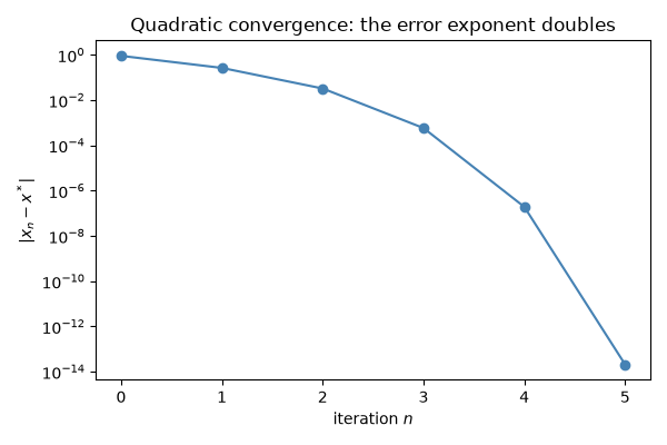
step 0: error = 9.05e-01  correct digits ~ 0.0
step 1: error = 2.65e-01  correct digits ~ 0.6
step 2: error = 3.26e-02  correct digits ~ 1.5
step 3: error = 5.85e-04  correct digits ~ 3.2
step 4: error = 1.92e-07  correct digits ~ 6.7
step 5: error = 2.09e-14  correct digits ~ 13.7
empirical order ~ 1.99