Horner’s method: evaluation, derivative, and deflation

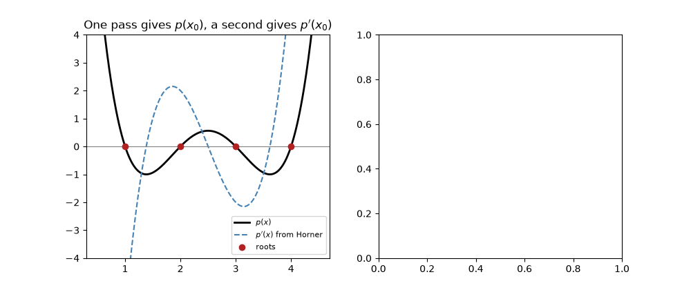
Horner’s 1819 scheme rewrites \(a_n x^n + \dots + a_0\) as nested multiplications, using \(n\) multiplications instead of the \(2n - 1\) of the term-by-term form. Its intermediate values are the coefficients of the quotient \(p(x) / (x - x_0)\), which gives the derivative for Newton’s method and lets a found root be divided out (“deflation”). This script finds all roots of a quartic that way and compares operation counts.

import matplotlib.pyplot as plt
import numpy as np

from mathematicskit.numerical_analysis import horner

Newton’s method with Horner evaluation, then deflation

p = np.array([1.0, -10.0, 35.0, -50.0, 24.0])  # (x-1)(x-2)(x-3)(x-4)
coeffs = p.copy()
roots = []
for _ in range(len(p) - 1):
    x = 0.0
    for _ in range(50):
        step = horner(coeffs, x)
        x_new = x - step.value / step.derivative
        if abs(x_new - x) < 1e-14:
            break
        x = x_new
    roots.append(x_new)
    coeffs = horner(coeffs, x_new).quotient  # deflate
print("roots found by Newton + deflation:", np.round(roots, 12))

t = np.linspace(0.5, 4.5, 300)
fig, (ax1, ax2) = plt.subplots(1, 2, figsize=(10, 4.2))
ax1.plot(t, [horner(p, ti).value for ti in t], "k", lw=2, label="$p(x)$")
ax1.plot(t, [horner(p, ti).derivative for ti in t], "--", color="steelblue", label="$p'(x)$ from Horner")
ax1.scatter(roots, np.zeros(4), color="firebrick", zorder=3, label="roots")
ax1.axhline(0.0, color="gray", lw=0.8)
ax1.set_ylim(-4, 4)
ax1.set_title("One pass gives $p(x_0)$, a second gives $p'(x_0)$")
ax1.legend(fontsize=8)

roots found by Newton + deflation: [1. 2. 3. 4.]

<matplotlib.legend.Legend object at 0x1196e2e40>

Operation counts

degrees = np.arange(1, 21)
ax2.plot(degrees, degrees, "o-", label="Horner: $n$ multiplications")
ax2.plot(degrees, 2 * degrees - 1, "s-", label="powers + terms: $2n - 1$")
ax2.plot(degrees, degrees * (degrees + 1) / 2, "^-", label="naive $a_k x^k$: $n(n+1)/2$")
ax2.set_xlabel("degree $n$")
ax2.set_ylabel("multiplications")
ax2.set_title("Horner's scheme is optimal")
ax2.legend(fontsize=8)
fig.tight_layout()

plt.show()