D’Alembert’s traveling waves on a plucked string

Jean le Rond d’Alembert (1747) showed that every solution of \(u_{tt} = c^2 u_{xx}\) is a sum of two waves moving in opposite directions, \(u = F(x - ct) + G(x + ct)\). A plucked string’s triangular bump therefore splits into two half-height copies that run apart, reflect upside down at the fixed ends, and recombine. This script compares d’Alembert’s formula with a leapfrog finite-difference string (mathematicskit.integrators.leapfrog_integrate()) run at Courant number 1, where the scheme reproduces d’Alembert’s solution exactly at the grid points.

import matplotlib.pyplot as plt
import numpy as np

from mathematicskit.pde import WaveEquation1D, dalembert_solution
from mathematicskit.pde.visualizers import plot_spacetime


def pluck(x):
    return np.maximum(0.0, 1.0 - np.abs(x - 0.3) / 0.1)


string = WaveEquation1D(pluck, n=201, c=1.0)
sol = string.solve(2.0, dt=string.dx, method="leapfrog", save_every=4)

The bump splits, reflects, and recombines

fig1, axes = plt.subplots(4, 1, figsize=(7, 7), sharex=True)
for ax, t in zip(axes, (0.0, 0.15, 0.5, 1.0), strict=False):
    k = int(np.argmin(np.abs(sol.t - t)))
    ax.plot(sol.x, sol.u[k], color="tab:blue", lw=2, label="leapfrog")
    ax.plot(sol.x, dalembert_solution(pluck, sol.x, sol.t[k], length=1.0), "k--", label="d'Alembert")
    ax.set_ylim(-1.1, 1.1)
    ax.set_ylabel(f"t = {sol.t[k]:.2f}")
axes[0].legend(fontsize=8, loc="upper right")
axes[-1].set_xlabel("$x$")
fig1.suptitle("Two half-height waves: d'Alembert's solution")
fig1.tight_layout()

errors = [np.max(np.abs(u - dalembert_solution(pluck, sol.x, t, length=1.0))) for t, u in zip(sol.t, sol.u, strict=False)]
print(f"max |leapfrog - d'Alembert| over the whole run: {max(errors):.2e}")

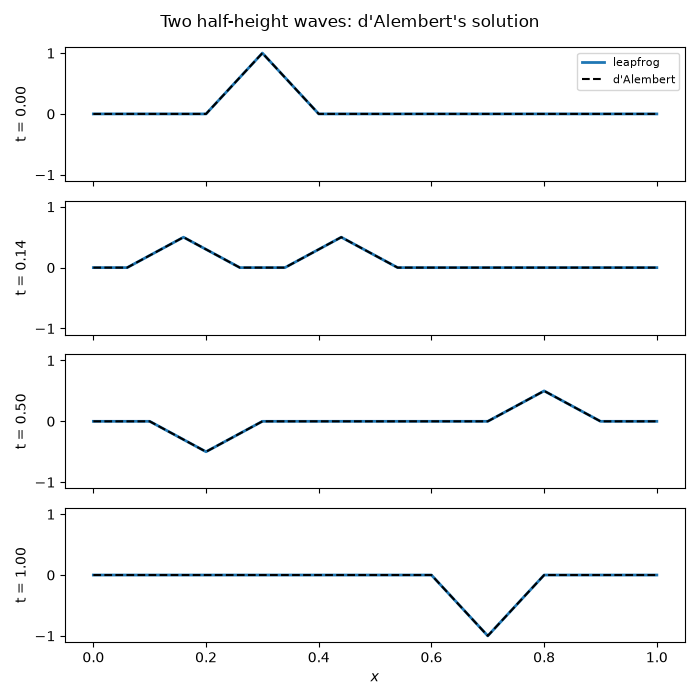
max |leapfrog - d'Alembert| over the whole run: 7.44e-15

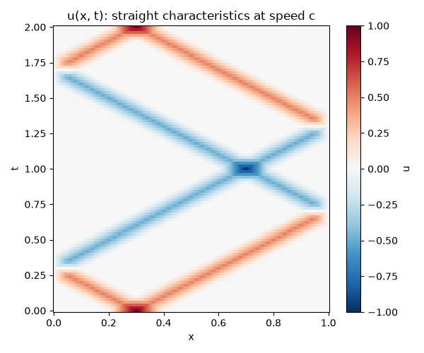
The characteristics in space-time

The waves travel along the lines \(x \pm ct = \text{const}\).

fig2, ax2 = plt.subplots(figsize=(6, 5))
plot_spacetime(sol, ax=ax2, cmap="RdBu_r")
ax2.set_title("u(x, t): straight characteristics at speed c")
fig2.tight_layout()

plt.show()