Fast convolution: the convolution theorem and the FFT

Stockham’s 1966 fast convolution: multiplying zero-padded FFT spectra gives the same linear convolution as the direct O(nm) sum, at O((n+m) log(n+m)) cost. Without the zero padding the product gives the circular convolution instead.

import matplotlib.pyplot as plt
import numpy as np

from mathematicskit.special_functions import circular_convolve, compare_convolution_methods, convolve_direct, convolve_fft

Same result, two algorithms

Smoothing a noisy step with a Gaussian kernel.

rng = np.random.default_rng(0)
x = np.concatenate([np.zeros(200), np.ones(200)]) + 0.2 * rng.normal(size=400)
kernel = np.exp(-0.5 * (np.arange(-30, 31) / 8.0) ** 2)
kernel /= kernel.sum()

direct = convolve_direct(x, kernel, mode="same")
fast = convolve_fft(x, kernel, mode="same")
print(f"max |direct - fft| = {np.max(np.abs(direct - fast)):.2e}")

fig, ax = plt.subplots()
ax.plot(x, lw=0.6, alpha=0.6, label="noisy step")
ax.plot(fast, lw=2, label="Gaussian-smoothed (FFT convolution)")
ax.legend()
ax.set_title("Convolution with a Gaussian kernel")

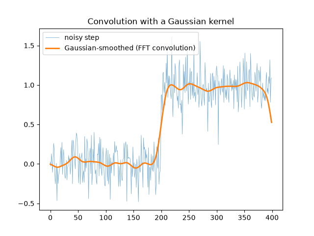
max |direct - fft| = 5.55e-16

Text(0.5, 1.0, 'Convolution with a Gaussian kernel')

Linear vs. circular convolution

The DFT product without padding wraps the tail of the linear convolution back onto its start.

a = np.array([1.0, 2.0, 3.0, 4.0])
h = np.array([1.0, 1.0, 0.0, 0.0])
print("linear  :", convolve_direct(a, h))
print("circular:", np.round(circular_convolve(a, h), 12))

linear  : [1. 3. 5. 7. 4. 0. 0.]
circular: [5. 3. 5. 7.]

O(nm) vs. O((n+m) log(n+m))

kernel_sizes = [8, 32, 128, 512, 2048, 8192]
direct_times, fft_times = [], []
for m in kernel_sizes:
    result = compare_convolution_methods(20000, m, seed=0)
    direct_times.append(result.direct_time)
    fft_times.append(result.fft_time)
    print(f"m={m:>5}: direct={result.direct_time * 1000:8.3f} ms, fft={result.fft_time * 1000:7.3f} ms, max error={result.max_error:.1e}")

fig, ax = plt.subplots()
ax.loglog(kernel_sizes, direct_times, "o-", label="direct: O(nm)")
ax.loglog(kernel_sizes, fft_times, "o-", label="FFT: O((n+m) log(n+m))")
ax.set_xlabel("kernel length m (signal length n = 20000)")
ax.set_ylabel("time (s)")
ax.set_title("Direct vs. FFT convolution")
ax.legend()

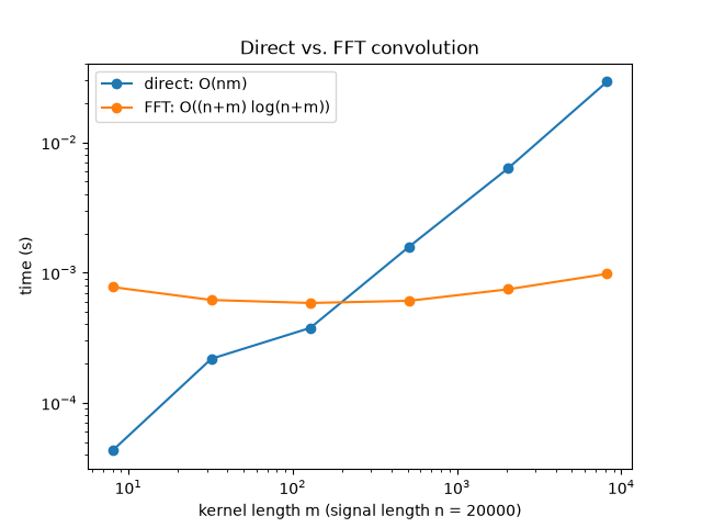
m=    8: direct=   0.043 ms, fft=  0.774 ms, max error=6.2e-15
m=   32: direct=   0.218 ms, fft=  0.616 ms, max error=1.4e-14
m=  128: direct=   0.376 ms, fft=  0.584 ms, max error=3.2e-14
m=  512: direct=   1.582 ms, fft=  0.607 ms, max error=6.4e-14
m= 2048: direct=   6.314 ms, fft=  0.744 ms, max error=1.4e-13
m= 8192: direct=  29.173 ms, fft=  0.977 ms, max error=3.8e-13

<matplotlib.legend.Legend object at 0x7fd7c13f8c20>