The Z-transform: poles, stability, and partial fractions

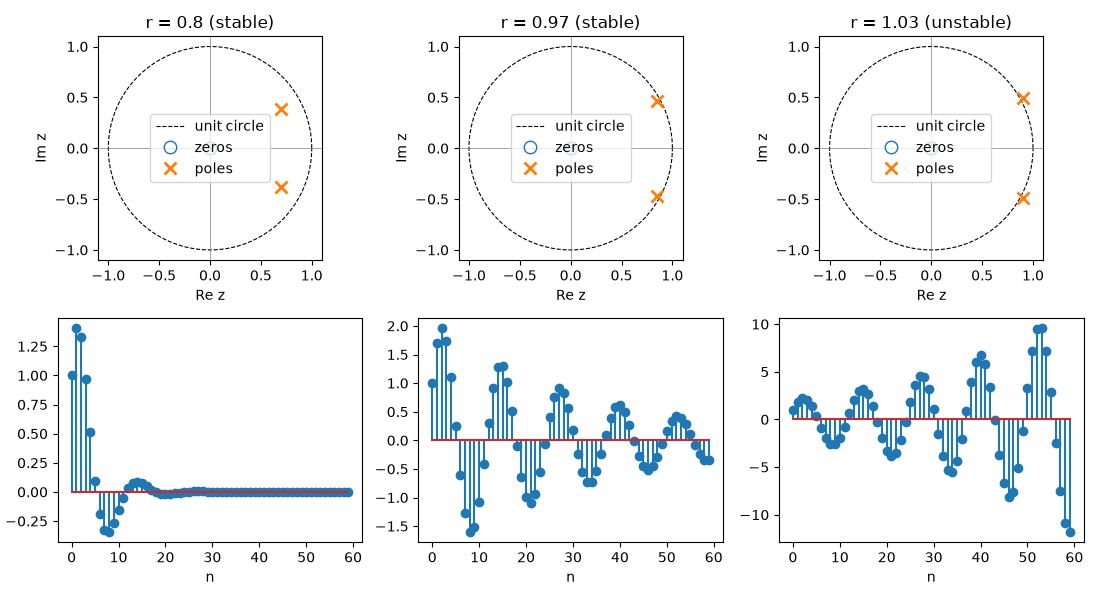
Ragazzini and Zadeh’s 1952 Z-transform turns a difference equation into a rational function H(z). Each pole p contributes a mode p^n to the impulse response, so poles inside the unit circle decay and a pole outside grows without bound. Partial fractions invert H(z) term by term.

import matplotlib.pyplot as plt
import numpy as np

from mathematicskit.special_functions import inverse_z_transform, poles_zeros, transfer_function, z_transform
from mathematicskit.special_functions.visualizers.plots import plot_pole_zero

Pole radius controls decay

H(z) = 1 / (1 - 2 r cos(w) z^-1 + r^2 z^-2) has poles r e^{+-iw}.

w = 0.5
fig, axes = plt.subplots(2, 3, figsize=(11, 6))
for col, r in enumerate((0.8, 0.97, 1.03)):
    a = [1.0, -2 * r * np.cos(w), r**2]
    result = poles_zeros([1.0], a)
    plot_pole_zero(result, ax=axes[0, col])
    axes[0, col].set_title(f"r = {r} ({'stable' if result.is_stable else 'unstable'})")
    axes[1, col].stem(inverse_z_transform([1.0], a, 60))
    axes[1, col].set_xlabel("n")
fig.tight_layout()

Inverse by partial fractions, including a repeated pole

1 / (1 - p z^-1)^2 inverts to (n + 1) p^n.

p = 0.8
n = np.arange(12)
h = inverse_z_transform([1.0], np.poly([p, p]), 12)
print("partial fractions:", np.round(h, 6))
print("(n + 1) p^n      :", np.round((n + 1) * p**n, 6))

partial fractions: [1.       1.6      1.92     2.048    2.048    1.96608  1.835008 1.677722
 1.509949 1.342177 1.181116 1.030792]
(n + 1) p^n      : [1.       1.6      1.92     2.048    2.048    1.96608  1.835008 1.677722
 1.509949 1.342177 1.181116 1.030792]

The transform of the impulse response is H(z)

b, a = [1.0, 0.5], [1.0, -0.9, 0.2]
h = inverse_z_transform(b, a, 300)
z = 1.2 * np.exp(0.7j)
print(f"sum h[n] z^-n = {complex(z_transform(h, z)):.10f}")
print(f"B(z) / A(z)   = {complex(transfer_function(b, a, z)):.10f}")

sum h[n] z^-n = 1.5521843777-1.7910734500j
B(z) / A(z)   = 1.5521843777-1.7910734500j