Hashcash: proof of work you can verify in one hash (Back 1997)

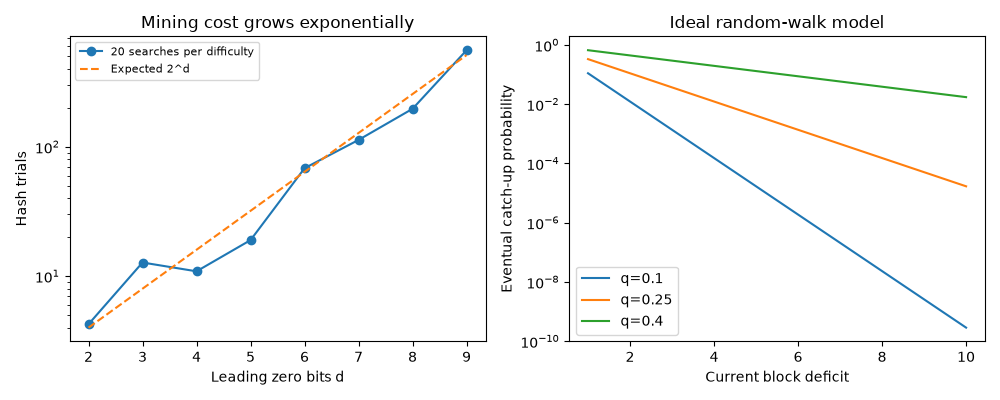
With d leading zero bits, a uniform hash succeeds with probability 2**(-d). The expected search is 2**d trials, but any one run can finish much earlier or later. Nonce search changes a commitment without changing the payload.

What to look for

Compare measured mining attempts with the average predicted by difficulty. Individual searches fluctuate: the average is not a deadline.

Read cells in order. An assert that produces no output has passed. The final exercise asks you to change an input and explain the result.

The history behind this experiment: Breakthroughs in Consensus. See Exercises: consensus for a worked solution to the exercise.

import matplotlib.pyplot as plt
import numpy as np

import blockchainkit as bk

difficulties = list(range(2, 10))
samples = []
for difficulty in difficulties:
    attempts = []
    for trial in range(20):
        block = bk.structures.Block(difficulty=difficulty, timestamp=trial)
        result = bk.consensus.mine(block, max_attempts=100_000)
        assert bk.consensus.valid_pow(result.block)
        attempts.append(result.attempts)
    samples.append(attempts)
print("Measured means:", [round(float(np.mean(row)), 1) for row in samples])

Measured means: [4.2, 12.8, 10.9, 19.0, 68.3, 113.1, 196.8, 558.5]

fig, axes = plt.subplots(1, 2, figsize=(10, 4))
means = np.mean(samples, axis=1)
axes[0].plot(difficulties, means, "o-", label="20 searches per difficulty")
axes[0].plot(
    difficulties,
    [bk.consensus.expected_trials(d) for d in difficulties],
    "--",
    label="Expected 2^d",
)
axes[0].set(
    yscale="log",
    xlabel="Leading zero bits d",
    ylabel="Hash trials",
    title="Mining cost grows exponentially",
)
axes[0].legend(fontsize=8)
for fraction in (0.1, 0.25, 0.4):
    deficits = list(range(1, 11))
    axes[1].plot(
        deficits,
        [bk.consensus.eventual_catch_up(fraction, z) for z in deficits],
        label=f"q={fraction}",
    )
axes[1].set(
    yscale="log",
    xlabel="Current block deficit",
    ylabel="Eventual catch-up probability",
    title="Ideal random-walk model",
)
axes[1].legend()
fig.tight_layout()

Exercise

Repeat with more trials and compare means and medians. The right plot assumes independent block discoveries and an infinite horizon; it is not Nakamoto’s Poisson confirmation calculation and omits propagation effects.