Heath-Jarrow-Morton: the drift condition

David Heath, Robert Jarrow and Andrew Morton (1992) modelled the whole forward curve at once,

\[df(t, T) = \alpha(t, T)\,dt + \sigma(t, T)\,dW(t),\]

starting from today’s market curve. Their central result is that the drift is not free: discounted bond prices are martingales only if

\[\alpha(t, T) = \sigma(t, T)\int_t^T \sigma(t, u)\,du.\]

The volatility is the whole model; a constant \(\sigma\) is Ho-Lee and \(\sigma e^{-a(T-t)}\) is Hull-White. Leaving the drift out creates an arbitrage, visible as a mispricing of the very bonds the simulation started from.

import matplotlib.pyplot as plt
import numpy as np

from financialkit.fixed_income import NelsonSiegelCurve
from financialkit.interest_rate_models import hjm_drift, simulate_hjm
from financialkit.interest_rate_models.visualizers import plot_forward_curves

curve = NelsonSiegelCurve(0.05, -0.02, 0.01, 2.0)
sigma, a = 0.015, 0.1

The drift each volatility requires

T = np.linspace(0, 20, 81)
fig, axes = plt.subplots(1, 3, figsize=(15, 4))
vols = {
    "constant (Ho-Lee)": lambda t, T: sigma,
    "exponential (Hull-White)": lambda t, T: sigma * np.exp(-a * (T - t)),
    "humped": lambda t, T: sigma * (1 + 2 * (T - t)) * np.exp(-0.5 * (T - t)),
}
for name, vol in vols.items():
    axes[0].plot(T, 1e4 * hjm_drift(vol, 0.0, T), label=name)
axes[0].set_xlabel("maturity T (years)")
axes[0].set_ylabel(r"$\alpha(0, T)$ (bp per year)")
axes[0].legend()

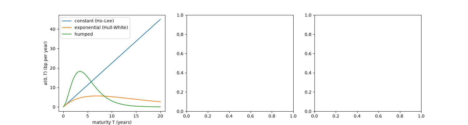
<matplotlib.legend.Legend object at 0x11a4fe120>

Simulated forward curves

res = simulate_hjm(curve, sigma, a, horizon=10.0, n_steps=50, n_paths=3000, rng=0)
plot_forward_curves(res, path=0, every=5, ax=axes[1])
axes[1].set_title("one path of f(t, T), t = 0, 1, ..., 9")

Text(0.5, 1.0, 'one path of f(t, T), t = 0, 1, ..., 9')

With and without the drift condition

Re-price today’s bonds by averaging the simulated discount factors.

wrong = simulate_hjm(curve, sigma, a, horizon=10.0, n_steps=50, n_paths=3000, drift_condition=False, rng=0)
exact = curve.discount(res.times)
for r, name in ((res, "HJM drift"), (wrong, "zero drift")):
    p, se = r.bond_prices()
    axes[2].fill_between(res.times, 1e4 * (p - exact - 2 * se), 1e4 * (p - exact + 2 * se), alpha=0.3)
    axes[2].plot(res.times, 1e4 * (p - exact), label=name)
    print(f"{name}: 10y bond off by {1e4 * (p[-1] - exact[-1]):+.1f} bp of face ({(p[-1] - exact[-1]) / se[-1]:+.1f} standard errors)")
axes[2].axhline(0, color="k", lw=0.5)
axes[2].set_xlabel("maturity T (years)")
axes[2].set_ylabel("Monte Carlo - market price (bp of face)")
axes[2].legend()
fig.tight_layout()

plt.show()

HJM drift: 10y bond off by +17.1 bp of face (+0.8 standard errors)
zero drift: 10y bond off by +138.5 bp of face (+6.2 standard errors)