Feller’s boundary condition

William Feller (1951) classified the boundaries of diffusions such as the square-root process

\[dr = \kappa(\theta - r)\,dt + \sigma\sqrt{r}\,dW.\]

When \(2\kappa\theta \ge \sigma^2\) the pull towards \(\theta\) beats the noise near zero and the process never reaches it; below that the process touches zero and is reflected. The same ratio is the shape of the stationary gamma distribution, whose density diverges at zero when the condition fails. The CIR rate and the Heston variance live or die by it.

import matplotlib.pyplot as plt
import numpy as np
from scipy.stats import gamma

from financialkit.interest_rate_models import CIRModel, feller_condition

Paths on either side of the condition

Exact noncentral chi-square sampling, so any visit to zero is the process itself, not a discretisation artefact.

models = {"Feller holds (ratio 4)": CIRModel(0.04, 2.0, 0.04, 0.2), "Feller fails (ratio 0.32)": CIRModel(0.04, 1.0, 0.04, 0.5)}
fig, axes = plt.subplots(1, 3, figsize=(14, 4))
for ax, (name, m) in zip(axes[:2], models.items(), strict=True):
    times, r = m.simulate(5.0, 500, 2000, rng=0)
    ax.plot(times, 100 * r[:8].T, lw=0.7)
    ax.set_title(name)
    ax.set_xlabel("t (years)")
    ax.set_ylabel("short rate (%)")
    near_zero = np.mean(r.min(axis=1) < 1e-5)
    print(f"{name}: {100 * near_zero:.1f}% of paths come within 0.001% of zero")

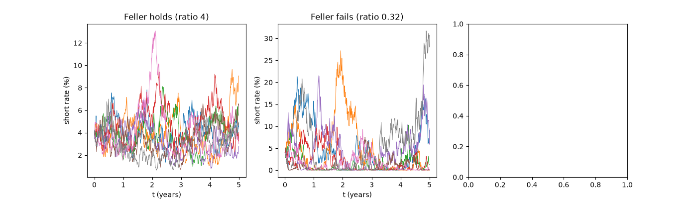
Feller holds (ratio 4): 0.0% of paths come within 0.001% of zero
Feller fails (ratio 0.32): 97.8% of paths come within 0.001% of zero

The stationary density

x = np.linspace(1e-4, 0.15, 400)
for sigma in (0.08, 0.2, 0.28, 0.4):
    m = CIRModel(0.04, 1.0, 0.04, sigma)
    shape, scale = m.stationary_shape_scale()
    axes[2].plot(100 * x, gamma.pdf(x, shape, scale=scale) / 100, label=f"ratio {feller_condition(1.0, 0.04, sigma):.2f}")
axes[2].set_ylim(0, 0.6)
axes[2].set_xlabel("short rate (%)")
axes[2].set_ylabel("stationary density (per %)")
axes[2].legend(title=r"$2\kappa\theta/\sigma^2$")
fig.tight_layout()

plt.show()