Broadie-Glasserman pathwise Greeks

Mark Broadie and Paul Glasserman (1996) differentiated each simulated payoff with respect to the parameter and averaged:

\[\Delta = E\left[e^{-rT}\mathbf 1\{S_T > K\}\frac{S_T}{S}\right], \qquad \mathcal V = E\left[e^{-rT}\mathbf 1\{S_T > K\} S_T(\sqrt T Z - \sigma T)\right].\]

Interchanging derivative and expectation is valid when the payoff is Lipschitz, as a call’s is. The estimator is then far less noisy than the likelihood ratio on the same paths, but it has nothing to say about a digital, or about the gamma of a call, whose derivatives jump.

import matplotlib.pyplot as plt
import numpy as np

from financialkit.monte_carlo import likelihood_ratio_greeks, pathwise_greeks
from financialkit.options import black_scholes_greeks

S, K, T, r, sigma = 100.0, 100.0, 0.5, 0.03, 0.25
exact = black_scholes_greeks(S, K, T, r, sigma)

Pathwise against likelihood ratio, on common random numbers

z = np.random.default_rng(0).standard_normal(100_000)
pw, lr = pathwise_greeks(S, K, T, r, sigma, z=z), likelihood_ratio_greeks(S, K, T, r, sigma, z=z)
for name in ("delta", "vega"):
    print(
        f"{name}: exact {getattr(exact, name):.4f}; pathwise {getattr(pw, name):.4f} +/- {getattr(pw, name + '_se'):.4f}; "
        f"likelihood ratio {getattr(lr, name):.4f} +/- {getattr(lr, name + '_se'):.4f}"
    )

delta: exact 0.5688; pathwise 0.5670 +/- 0.0018; likelihood ratio 0.5674 +/- 0.0043
vega: exact 27.7893; pathwise 27.7650 +/- 0.1619; likelihood ratio 27.7868 +/- 0.5900

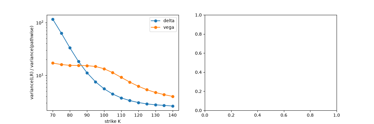
The variance advantage across strikes

strikes = np.linspace(70, 140, 15)
ratio = {"delta": [], "vega": []}
for k in strikes:
    p, l = pathwise_greeks(S, k, T, r, sigma, z=z), likelihood_ratio_greeks(S, k, T, r, sigma, z=z)
    for name in ratio:
        ratio[name].append((getattr(l, name + "_se") / getattr(p, name + "_se")) ** 2)
fig, axes = plt.subplots(1, 2, figsize=(12, 4))
for name, v in ratio.items():
    axes[0].semilogy(strikes, v, "o-", label=name)
axes[0].set_xlabel("strike K")
axes[0].set_ylabel("variance(LR) / variance(pathwise)")
axes[0].legend()

<matplotlib.legend.Legend object at 0x1125201a0>

Pathwise deltas converge with the paths

ns = 1000 * 4 ** np.arange(5)
g = [pathwise_greeks(S, K, T, r, sigma, n_paths=n, rng=n) for n in ns]
axes[1].errorbar(ns, [x.delta for x in g], yerr=[2 * x.delta_se for x in g], fmt="o", capsize=3, label="pathwise delta")
axes[1].axhline(exact.delta, color="k", label="Black-Scholes")
axes[1].set_xscale("log")
axes[1].set_xlabel("paths")
axes[1].legend()
fig.tight_layout()
plt.show()