Giles multilevel Monte Carlo

Pricing with a discretised SDE has two errors: the bias of the time step and the statistical error. Balancing them with Euler’s scheme costs \(O(\varepsilon^{-3})\). Michael Giles (2008), borrowing the idea of multigrid (and of Heinrich’s multilevel integration), wrote the finest approximation as a telescoping sum,

\[E[P_L] = E[P_0] + \sum_{l=1}^{L} E[P_l - P_{l-1}],\]

and simulated each correction on coupled fine and coarse paths that share Brownian increments. The corrections have small variance, so most samples go to the cheap levels and the cost falls to \(O(\varepsilon^{-2}(\log\varepsilon)^2)\). The paths are Euler solutions from financialkit.integrators.euler_maruyama().

import matplotlib.pyplot as plt
import numpy as np

from financialkit.monte_carlo import multilevel_monte_carlo
from financialkit.monte_carlo.visualizers import plot_mlmc
from financialkit.options import black_scholes_price

S, K, T, r, sigma = 100.0, 100.0, 1.0, 0.05, 0.2
exact = black_scholes_price(S, K, T, r, sigma)

Level diagnostics

The variance of \(P_l - P_{l-1}\) falls by about 2 per level, and so does the mean (the weak error of Euler).

res = multilevel_monte_carlo(S, K, T, r, sigma, eps=0.02, rng=0)
print(f"MLMC {res.estimate:.4f} +/- {res.std_error:.4f} (target RMSE {res.target_rmse}), Black-Scholes {exact:.4f}")
print("samples per level:", res.level_samples.tolist())
fig, axes = plt.subplots(1, 3, figsize=(16, 4))
plot_mlmc(res, axes=axes[:2])

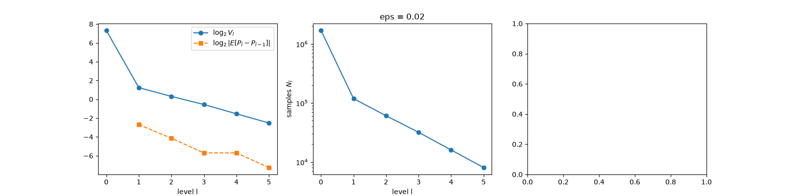
MLMC 10.4453 +/- 0.0141 (target RMSE 0.02), Black-Scholes 10.4506
samples per level: [1697090, 118731, 60806, 31872, 16009, 8055]

array([<Axes: xlabel='level l'>,
       <Axes: title={'center': 'eps = 0.02'}, xlabel='level l', ylabel='samples $N_l$'>],
      dtype=object)

Cost against accuracy

\(\varepsilon^2 \times\) cost grows only logarithmically for MLMC, like \(1/\varepsilon\) for standard Monte Carlo.

eps = np.array([0.2, 0.1, 0.05, 0.03, 0.02])
runs = [multilevel_monte_carlo(S, K, T, r, sigma, eps=e, rng=i) for i, e in enumerate(eps)]
axes[2].loglog(eps, eps**2 * np.array([x.cost for x in runs]), "o-", label="multilevel")
axes[2].loglog(eps, eps**2 * np.array([x.standard_mc_cost for x in runs]), "s-", label="standard MC")
axes[2].set_xlabel(r"target RMSE $\varepsilon$")
axes[2].set_ylabel(r"$\varepsilon^2 \times$ cost (time steps)")
axes[2].legend()
fig.tight_layout()
plt.show()