Halton sequences

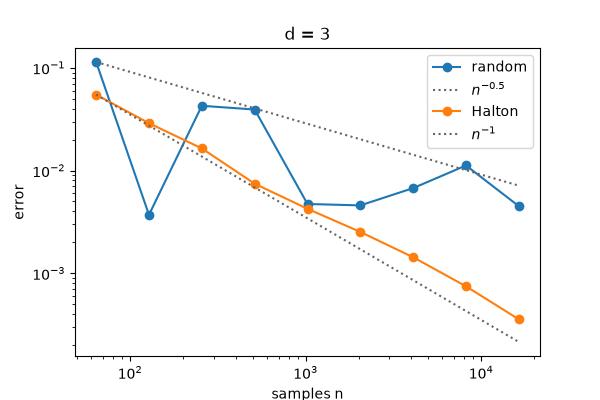
Johannes van der Corput (1935) built a one-dimensional sequence that fills the unit interval evenly by reflecting the binary digits of \(k\) about the radix point: 1/2, 1/4, 3/4, 1/8, 5/8, … John Halton (1960) took one such radical-inverse sequence per coordinate, in distinct prime bases, to fill the \(d\)-dimensional cube. The points are deterministic, yet integrate far better than random ones in low dimension, with an error close to \((\log n)^d / n\).

import matplotlib.pyplot as plt
import numpy as np

from financialkit.monte_carlo import halton, van_der_corput
from financialkit.monte_carlo.visualizers import plot_error_convergence, plot_point_set

Van der Corput fills the largest gap

print("base 2:", van_der_corput(8).tolist())
print("base 3:", np.round(van_der_corput(8, base=3), 4).tolist())

fig, axes = plt.subplots(1, 4, figsize=(17, 4))
x = van_der_corput(16)
axes[0].scatter(x, np.arange(16), c=np.arange(16))
axes[0].set_xlabel("point")
axes[0].set_ylabel("index k")
axes[0].set_title("van der Corput, base 2")

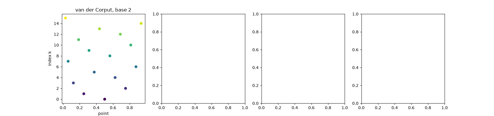
base 2: [0.5, 0.25, 0.75, 0.125, 0.625, 0.375, 0.875, 0.0625]
base 3: [0.3333, 0.6667, 0.1111, 0.4444, 0.7778, 0.2222, 0.5556, 0.8889]

Text(0.5, 1.0, 'van der Corput, base 2')

Halton points against random points

plot_point_set(np.random.default_rng(0).random((256, 2)), ax=axes[1], title="256 random points")
plot_point_set(halton(256, 2), ax=axes[2], title="256 Halton points (bases 2, 3)")

<Axes: title={'center': '256 Halton points (bases 2, 3)'}, xlabel='$u_{1}$', ylabel='$u_{2}$'>

Large neighbouring primes correlate

Coordinates 15 and 16 (bases 47 and 53) march in step for the first points; scrambling the digits breaks the pattern.

plot_point_set(halton(256, 16), ax=axes[3], dims=(14, 15), title="dims 15-16 (bases 47, 53)")

<Axes: title={'center': 'dims 15-16 (bases 47, 53)'}, xlabel='$u_{15}$', ylabel='$u_{16}$'>

Integration error

f = lambda u: np.prod(1 + (u - 0.5), axis=1)  # noqa: E731  integral 1
ns = 2 ** np.arange(6, 15)
fig, ax = plt.subplots(figsize=(6, 4))
mc = [abs(f(np.random.default_rng(n).random((n, 3))).mean() - 1) for n in ns]
ha = [abs(f(halton(n, 3)).mean() - 1) for n in ns]
plot_error_convergence(ns, mc, ax=ax, label="random", rates=(0.5,))
plot_error_convergence(ns, ha, ax=ax, label="Halton", rates=(1.0,))
ax.set_title("d = 3")
plt.show()