Crank-Nicolson

John Crank and Phyllis Nicolson (1947) averaged the explicit and implicit differences of the heat equation around the half step,

\[\frac{V^{n+1} - V^n}{\Delta\tau} = \tfrac12 \bigl(A V^{n+1} + A V^n\bigr),\]

which makes the scheme unconditionally stable and second-order accurate in time. Applied to the Black-Scholes equation it is the workhorse of finite-difference option pricing. Here CrankNicolson prices a call and its error falls by four each time both grids are halved.

import matplotlib.pyplot as plt
import numpy as np

from financialkit.options import black_scholes_price
from financialkit.pde_methods import CrankNicolson
from financialkit.pde_methods.visualizers import plot_grid_convergence, plot_value_surface

S, K, T, r, sigma = 100.0, 100.0, 1.0, 0.05, 0.2
exact = black_scholes_price(S, K, T, r, sigma)

res = CrankNicolson(200, 100, rannacher_steps=2).price(S, K, T, r, sigma)
print(f"Crank-Nicolson {res.price:.5f}, Black-Scholes {exact:.5f}")

Crank-Nicolson 10.44060, Black-Scholes 10.45058

The value surface, from the payoff at expiry back to today

fig, axes = plt.subplots(1, 2, figsize=(11, 4))
plot_value_surface(res, ax=axes[0], s_range=(40, 180))
axes[0].set_title("call value V(S, t)")

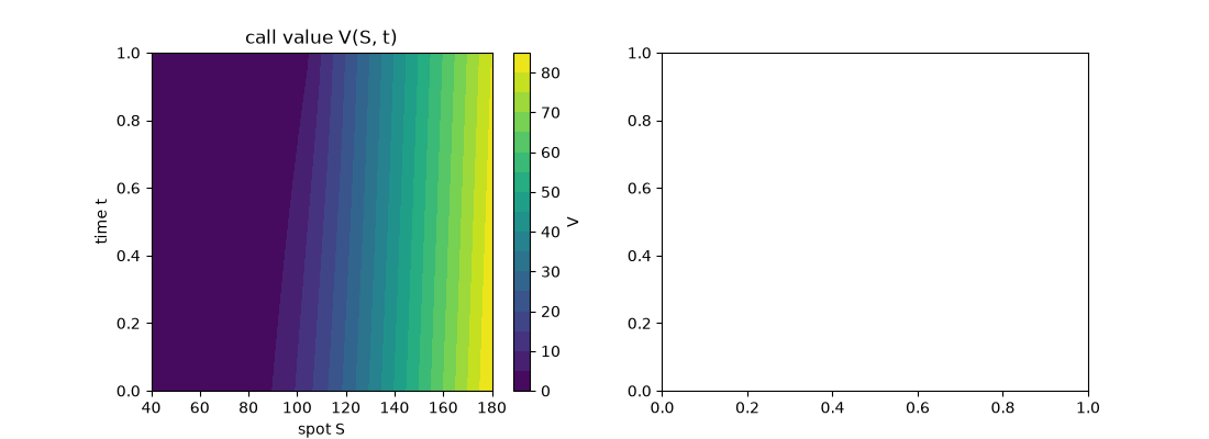
Text(0.5, 1.0, 'call value V(S, t)')

Second order in space and time together

ns = np.array([25, 50, 100, 200, 400])
errors = [abs(CrankNicolson(n, n, rannacher_steps=2, s_max=400.0).price(S, K, T, r, sigma).price - exact) for n in ns]
plot_grid_convergence(ns, errors, ax=axes[1], label="Crank-Nicolson, M = N = n", rates=(2.0,))
axes[1].set_title("error against grid size")
fig.tight_layout()
plt.show()