Schwartz: explicit finite differences

Eduardo Schwartz (1977) valued warrants, which no formula covered, by replacing the derivatives in the Black-Scholes equation with differences and stepping back from expiry one explicit step at a time:

\[V_i^{n+1} = V_i^n + \Delta\tau\,(a_i V_{i-1}^n + b_i V_i^n + c_i V_{i+1}^n).\]

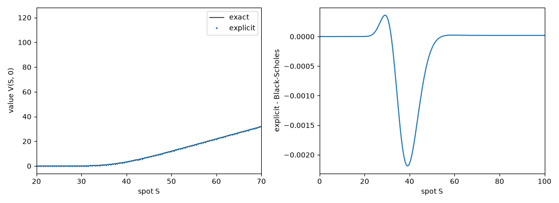
No linear system is solved, so each step is cheap, but the time step must stay below a limit set by the finest spot spacing. ExplicitScheme reproduces Hull’s Example 15.6 call, and its whole grid matches Black-Scholes.

import matplotlib.pyplot as plt

from financialkit.options import black_scholes_price
from financialkit.pde_methods import ExplicitScheme
from financialkit.pde_methods.visualizers import plot_value_profile

# Hull, 10th ed., Example 15.6
S, K, T, r, sigma = 42.0, 40.0, 0.5, 0.10, 0.20
res = ExplicitScheme(320, 2500, s_max=160.0).price(S, K, T, r, sigma)
print(f"explicit {res.price:.4f}, Black-Scholes {black_scholes_price(S, K, T, r, sigma):.4f}")
print(f"time step {res.stability.number:.2e} below the limit {res.stability.limit:.2e}: {res.stability.stable}")

explicit 4.7576, Black-Scholes 4.7594
time step 2.00e-04 below the limit 2.57e-04: True

The whole grid at once

fig, axes = plt.subplots(1, 2, figsize=(11, 4))
plot_value_profile(res, exact=black_scholes_price(res.S, K, T, r, sigma), ax=axes[0], xlim=(20, 70))
err = res.V - black_scholes_price(res.S, K, T, r, sigma)
axes[1].plot(res.S, err)
axes[1].set_xlim(0, 100)
axes[1].set_xlabel("spot S")
axes[1].set_ylabel("explicit - Black-Scholes")
fig.tight_layout()
plt.show()