Brennan-Schwartz: explicit schemes are trinomial trees

Brennan and Schwartz (1978) noticed that in \(x = \ln S\) the explicit scheme’s weights on the three neighbouring nodes sum to one and match the mean and variance of the log-price increment: the explicit scheme is a trinomial tree, and its stability condition is just the requirement that the weights be probabilities. With \(\Delta x = \sigma\sqrt{3\Delta t}\) the middle weight is 2/3, Hull’s standard tree. log_explicit_price() runs the scheme, and explicit_trinomial_probabilities() shows the weights turn negative exactly where the scheme becomes unstable.

import matplotlib.pyplot as plt
import numpy as np

from financialkit.options import CRRTree, black_scholes_price
from financialkit.pde_methods import explicit_trinomial_probabilities, log_explicit_price

S, K, T, r, sigma = 50.0, 50.0, 5 / 12, 0.10, 0.40
dt = T / 200
p = explicit_trinomial_probabilities(sigma, r, dt, sigma * np.sqrt(3 * dt))
print(f"p_down {p.p_down:.4f}, p_mid {p.p_mid:.4f}, p_up {p.p_up:.4f}, total {p.total:.4f}")

p_down 0.1660, p_mid 0.6667, p_up 0.1673, total 1.0000

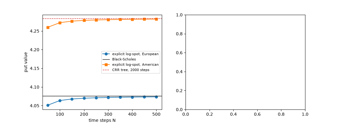
The scheme prices like a tree: European and American puts

ns = np.arange(50, 501, 50)
eu = [log_explicit_price(S, K, T, r, sigma, option_type="put", n_time=n).price for n in ns]
am = [log_explicit_price(S, K, T, r, sigma, option_type="put", american=True, n_time=n).price for n in ns]
crr = CRRTree(2000).price(S, K, T, r, sigma, option_type="put", american=True).price

fig, axes = plt.subplots(1, 2, figsize=(11, 4))
axes[0].plot(ns, eu, "o-", label="explicit log-spot, European")
axes[0].axhline(black_scholes_price(S, K, T, r, sigma, option_type="put"), color="k", lw=1, label="Black-Scholes")
axes[0].plot(ns, am, "s-", label="explicit log-spot, American")
axes[0].axhline(crr, color="C3", lw=1, ls="--", label="CRR tree, 2000 steps")
axes[0].set_xlabel("time steps N")
axes[0].set_ylabel("put value")
axes[0].legend(fontsize=8)

<matplotlib.legend.Legend object at 0x116d7e3c0>

Negative probabilities are instability

lam = np.linspace(0.2, 1.6, 50)
p_mid = [explicit_trinomial_probabilities(sigma, r, dt, sigma * np.sqrt(dt / l)).p_mid for l in lam]
axes[1].plot(lam, p_mid)
axes[1].axhline(0.0, color="k", lw=0.8)
axes[1].axvline(1.0, color="C3", ls="--", label="stability limit")
axes[1].set_xlabel(r"diffusion number $\sigma^2 \Delta t / \Delta x^2$")
axes[1].set_ylabel("middle weight p_mid")
axes[1].legend()
fig.tight_layout()
plt.show()