Laasonen’s implicit scheme

Pentti Laasonen (1949) evaluated the space derivatives of the heat equation at the new time level, \((I - \Delta\tau A) V^{n+1} = V^n\). Every step is then a linear solve, but no step is too large: the scheme is stable and monotone for any \(\Delta\tau\), at the price of first-order accuracy in time. 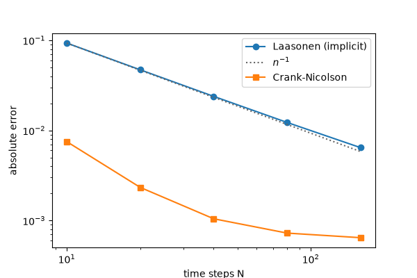ImplicitScheme shows both sides: a large step that would wreck the explicit scheme gives a sensible answer, and halving the step halves the error.

import matplotlib.pyplot as plt
import numpy as np

from financialkit.options import black_scholes_price
from financialkit.pde_methods import CrankNicolson, ImplicitScheme, explicit_stability
from financialkit.pde_methods.visualizers import plot_grid_convergence

S, K, T, r, sigma = 100.0, 100.0, 1.0, 0.05, 0.2
exact = black_scholes_price(S, K, T, r, sigma, option_type="put")

A time step 400 times the explicit limit

res = ImplicitScheme(400, 10).price(S, K, T, r, sigma, option_type="put")
limit = explicit_stability(res.S, 1.0, sigma, r).limit
print(f"explicit limit {limit:.2e}, implicit step {T / 10:.2e}")
print(f"implicit put with 10 steps {res.price:.4f}, Black-Scholes {exact:.4f}")

explicit limit 1.63e-04, implicit step 1.00e-01
implicit put with 10 steps 5.4785, Black-Scholes 5.5735

First order in time, against Crank-Nicolson’s second

ns = np.array([10, 20, 40, 80, 160])
imp = [abs(ImplicitScheme(800, n, s_max=400.0).price(S, K, T, r, sigma, option_type="put").price - exact) for n in ns]
cn = [abs(CrankNicolson(800, n, rannacher_steps=2, s_max=400.0).price(S, K, T, r, sigma, option_type="put").price - exact) for n in ns]
fig, ax = plt.subplots(figsize=(6, 4))
plot_grid_convergence(ns, imp, ax=ax, label="Laasonen (implicit)", rates=(1.0,))
ax.loglog(ns, cn, "s-", label="Crank-Nicolson")
ax.set_xlabel("time steps N")
ax.legend()
plt.show()